
Here is a brief summary of the properties of Bessel functions. It is roughly a summary of Chapter 6 of Bowman (1958). They will be necessary when considering Kepler’s equations (equations of elliptical motion) and the motion of electrons bound to atomic nuclei.
Bessel Functions
The function expressed by the infinite series below is called the 0th order Bessel function of the first kind.
\[ \small \begin{align*} J_0(x) & = 1-\frac{x^2}{2^2} + \frac{x^4}{2^2\cdot4^2}-\frac{x^6}{2^2\cdot4^2\cdot6^2}\cdots \\ & = \sum_{m=0}^\infty \frac{(-1)^m}{m!\Gamma(m+1)}\left(\frac{x}{2}\right)^{2m} \end{align*} \]
Where \(\small \Gamma(x)\) is the Gamma function. Generalized,
\[ \small \begin{align*} J_n(x) & = \frac{x^n}{2^nn!}\left(1-\frac{x^2}{2(2n+2)} + \frac{x^4}{2\cdot4(2n+2)(2n+4)}\cdots\right) \\ & = \sum_{m=0}^\infty \frac{(-1)^m}{m!\Gamma(m+n+1)}\left(\frac{x}{2}\right)^{2m+n} \end{align*} \]
is defined as the \(\small n\)-th order Bessel function. There is a relationship:
\[ \small \begin{align*} &\frac{d}{dx}\left\{x^nJ_n(x) \right\} = x^n J_{n-1}(x) \\
&\frac{d}{dx}\left\{\frac{J_n(x)}{x^n} \right\} = – \frac{J_{n+1}(x)}{x^n} \end{align*} \]
between Bessel functions. These can also be represented as:
\[ \small \frac{dJ_n(x)}{dx} = J_{n-1}(x)-\frac{n}{x}J_n(x)= -J_{n+1}(x)+\frac{n}{x}J_n(x). \]
From this formula we get
\[ \small \frac{dJ_n(x)}{dx} = \frac{J_{n-1}(x)-J_{n+1}(x)}{2}. \]
The Bessel functions are the solutions of the ordinary differential equation:
\[ \small x^2\frac{d^2y}{dx^2} + x\frac{dy}{dx}+(x^2 – n^2)y = 0. \]
This differential equation is called the \(\small n\)-th order Bessel equation. \(\small J_n(x)\) can also be expressed as the following integral, which is called the Bessel integral.
\[ \small J_n(x) = \frac{1}{\pi}\int_0^{\pi} \cos(n\theta-x\sin\theta)d\theta= \frac{1}{2\pi}\int_0^{2\pi} \cos(n\theta-x\sin\theta)d\theta \]
The Bessel equation has
\[ \small Y_n(x) = \frac{J_n(x) \cos n\pi-J_{-n}(x)}{\sin n\pi} \]
as a solution in addition to the Bessel function of the first kind \(\small J_n(x)\). This function is called the Bessel function of the second kind (when \(\small n\) is an integer, the numerator and denominator become 0, so it is necessary to calculate the limit). The general solution to the Bessel equation is expressed as a linear combination of \(\small J_n(x)\) and \(\small Y_n(x)\).
When we actually calculate the graph, it looks like this:
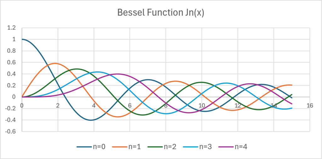
You can see that it fluctuates periodically like a trigonometric function.
Modified Bessel Functions
The solution of the equation obtained by modifying the Bessel equation to
\[ \small x^2\frac{d^2y}{dx^2} + x\frac{dy}{dx}-(x^2 + n^2)y = 0 \]
is called the modified Bessel functions. There are also two types, each defined as:
\[ \small \begin{align*} &I_n(x) = i^{-n}J(ix) = \sum_{m=0}^\infty \frac{1}{m!\Gamma(m+n+1)}\left(\frac{x}{2}\right)^{2m+n} \\ &K_n(x) = \frac{\pi}{2}\frac{I_{-n}(x)-I_{n}(x)}{\sin n\pi} \end{align*} \]
(for \(\small K_n(x)\), the limit needs to be calculated if \(\small n\) is an integer). Unlike the original Bessel functions, these are the functions that increases monotonically like an exponential function.
Another variation is the solution to
\[ \small x^2\frac{d^2y}{dx^2} + 2x\frac{dy}{dx}+(x^2 – n(n+1))y = 0, \]
called the spherical Bessel functions. It is probably well known that this form is an equation that appears in the Schrödinger equation (although I don’t know what problem it is). Each is defined by:
\[ \small j_n(x) = \sqrt{\frac{\pi}{2x}}J_{n+1/2}(x) \\
\small y_n(x) = \sqrt{\frac{\pi}{2x}}Y_{n+1/2}(x). \]
Bessel Function Series
There are numerous formulas for calculating series related to Bessel functions, but only the basic ones are shown here.
\[ \small \begin{align*} \exp\left(\frac{1}{2}x\left(t-\frac{1}{t} \right)\right) &= \sum_{n=-\infty}^\infty t^nJ_n(x) \\ & = J_0(x)+\sum_{n=1}^\infty (t^n+(-1)^nt^{-n})J_n(x) \end{align*} \]
For this type of exponential function, the coefficients of the Taylor expansion correspond to the Bessel functions. By substituting \(\small t\) to \(\small e^{i\theta}\),
\[ \small \begin{align*} \exp\left(ix\sin\theta \right)&= J_0(x)+\sum_{n=1}^\infty (e^{in\theta}+(-1)^nt^{-in\theta})J_n(x) \\ &= J_0(x)+2\sum_{n=1}^\infty \cos(2n\theta)J_{2n}(x)+2i\sum_{n=0}^\infty \sin((2n+1)\theta)J_{2n+1}(x) \end{align*} \]
can be obtained. This is apparently called Jacobi expansion. From this formula, we can obtain the following series:
\[ \small \begin{align*} &\cos(x\sin\theta) = J_0(x)+2\sum_{n=1}^\infty \cos(2n\theta)J_{2n}(x) \\ &\sin(x\sin\theta) =2\sum_{n=0}^\infty \sin((2n+1)\theta)J_{2n+1}(x) \\ &\cos(x\cos\theta) = J_0(x)+2\sum_{n=1}^\infty (-1)^n\cos(2n\theta)J_{2n}(x) \\ &\sin(x\cos\theta) =2\sum_{n=0}^\infty (-1)^n\sin((2n+1)\theta)J_{2n+1}(x). \end{align*} \]
Finally, any function \(\small f(x)\) defined on \(\small 0<x<1\) can be approximated by
\[ \small \begin{align*} &f(x) = \sum_{i=1}^\infty A_iJ_n(x\alpha_i) \\ &A_i = \frac{2}{J_{n+1}^2(\alpha_i)}\int_0^1 xf(x)J_n(x\alpha_i)dx, \end{align*} \]
if the positive solutions that satisfy \(\small J_n(x)=0\) are expressed in order of decreasing size as \(\small \alpha_1,\alpha_2,\cdots\). This is a type of Fourier expansion called the Fourier-Bessel expansion.
Reference
[1] Bowman, Frank, Introduction to Bessel Functions, Dover Publication Inc., 1958.
[2] Watson, George N., A Treatise on the Theory of Bessel Functions Second Edition, Cambridge University Press, 1944.


Comments