Schrödinger Equation in the Free State (3 Dimensions)

Gaussian Wave Packet Model

In a previous post:

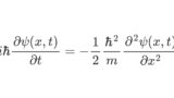
we mentioned that the solution to the one-dimensional free-state Schrödinger equation:

\[ \small \begin{align*} &i \hbar\frac{\partial \psi(x,t)}{\partial t} =-\frac{1}{2} \frac{\hbar^2}{m} \frac{\partial^2 \psi(x,t)}{\partial x^2} \\ &\psi(x,0) = \frac{1}{\sigma^{1/2}\pi^{1/4}} \exp\left(-\frac{x^2}{2\sigma^2}\right) \exp \left( \frac{i}{\hbar} \bar{p} x \right) \end{align*} \]

where the coordinate uncertainties follow a normal distribution is given by

\[ \small \begin{align*} \psi(x,t) \; & = \frac{1}{\pi^{1/4}\sigma^{1/2}} \frac{1}{\left( 1+\frac{i \hbar t}{m\sigma^2} \right)^{1/2}} \small \exp \left(-\frac{\left( x-\frac{\bar{p}}{m}t \right)^2}{2 \sigma^2 \left(1 + \left(\frac{\hbar t}{m\sigma^2} \right)^2 \right)} \right) \\ &\small \quad\;\times \exp \left(i \left\{ \frac{\bar{p}}{\hbar}x-\frac{\bar{p}^2 t}{2m \hbar} + \frac{\hbar t \left( x-\frac{\bar{p}}{m}t \right)^2}{2 m \sigma^4 \left(1 + \left( \frac{\hbar t}{m\sigma^2} \right)^2 \right)} \right\} \right). \end{align*} \]

Here, \(\small \sigma\) is a parameter that represents the uncertainty of the coordinates. The purpose of this article is to extend this to the three-dimensional case. However, among general quantum mechanics textbooks, there are quite a few that start presenting strange solutions (spherical wave solutions or solutions using spherical harmonic functions by analogy with Coulomb potential) as soon as they reach three dimensions. This is thought to be due to the failure to set appropriate boundary conditions. In this article, we will derive a solution when considering a Gaussian wave packet model (white noise model) as in the one-dimensional case.

 If it can be assumed that the uncertainties in the coordinates along each coordinate axis are independent and of the same order of magnitude (if the probability distribution can be assumed to be spherically symmetric), the boundary condition along each coordinate axis can be set to

\[ \small \psi(q_\mu,0) = \frac{1}{\sigma^{1/2}\pi^{1/4}} \exp\left(-\frac{q_\mu^2}{2\sigma^2}\right) \exp \left( \frac{i}{\hbar} \bar{p}_\mu x \right), \quad \mu=x,y,z. \]

Since the coordinates are assumed to be independent, the three-dimensional boundary condition can be expressed as the product of these wave functions and denoted as:

\[ \small \begin{align*} \psi(x,y,z,0) &= \psi(x, 0)\:\psi(y, 0)\:\psi(z, 0) \\ &=\frac{1}{\sigma^{3/2}\pi^{3/4}} \exp\left(-\frac{x^2+y^2+z^2}{2\sigma^2}\right) \exp \left( \frac{i}{\hbar} \left(\bar{p}_x x+\bar{p}_y y+\bar{p}_z z \right) \right). \end{align*} \]

Since the free state Schrödinger equation is \(\small V=0\),

\[ \small \begin{align*} &i \hbar\frac{\partial \psi(x,y,z,t)}{\partial t} = – \frac{1}{2}\frac{\hbar^2}{m} \left(\frac{\partial^2}{\partial x^2}+\frac{\partial^2 }{\partial y^2}+\frac{\partial^2 }{\partial z^2} \right)\psi(x,y,z,t) \\ &\psi(x,y,z,0) = \frac{1}{\sigma^{3/2}\pi^{3/4}} \exp\left(-\frac{x^2+y^2+z^2}{2\sigma^2}\right) \exp \left( \frac{i}{\hbar} \left(\bar{p}_x x+\bar{p}_y y+\bar{p}_z z \right) \right) \end{align*} \]

is the three-dimensional free-state Schrödinger equation. Since there is no potential, on average the quantum will either remain at its initial coordinates or move in a straight line with some uncertainty, and we can make the assumption that the expected value of the momentum in each coordinate direction is constant.

 Although the problem formulation is a little more complicated, finding a solution should not be too difficult. Since it was assumed that the probability distribution on each coordinate axis was independent, the solution is considered to be

\[ \small \psi(x,y,z,t) = \psi(x,t)\:\psi(y,t)\:\psi(z,t). \]

Hence, using the solution of the one-dimensional free-state Schrödinger equation, we can infer that

\[ \small \begin{align*} \psi(x,y,z,t) \; & = \frac{1}{\pi^{3/4}\sigma^{3/2}} \frac{1}{\left( 1+\frac{i \hbar t}{m\sigma^2} \right)^{3/2}} \small \exp \left(- \frac{\left(x-\frac{\bar{p}_x}{m}t \right)^2+\left(y-\frac{\bar{p}_y}{m}t \right)^2+\left(z-\frac{\bar{p}_z}{m}t \right)^2}{2 \sigma^2 \left(1 + \left(\frac{\hbar t}{m\sigma^2} \right)^2 \right)} \right) \\ &\small \quad\;\times \exp \left(i \left\{ \frac{\bar{p}_xx+\bar{p}_yy+\bar{p}_zz}{\hbar}-\frac{(\bar{p}_x^2+\bar{p}_y^2+\bar{p}_z^2) t}{2m \hbar} \right\} \right) \\ &\small \quad\;\times \exp \left(i \left\{\hbar t\frac{ \left(x-\frac{\bar{p}_x}{m}t \right)^2+\left(y-\frac{\bar{p}_y}{m}t \right)^2+\left(z-\frac{\bar{p}_z}{m}t \right)^2}{2 m \sigma^4 \left(1 + \left( \frac{\hbar t}{m\sigma^2} \right)^2 \right)} \right\} \right) \end{align*} \]

is a solution to the three-dimensional Schrödinger equation. Expressed as a stochastic process, it is

\[ \small \begin{align*} & x(t) \sim N\left(\frac{\bar{p}_x}{m}t,\; \frac{\sigma^2}{2}+\frac{\hbar^2}{2m^2\sigma^2}t^2\right) \\ & y(t) \sim N\left(\frac{\bar{p}_y}{m}t,\; \frac{\sigma^2}{2}+\frac{\hbar^2}{2m^2\sigma^2}t^2\right) \\ & z(t) \sim N\left(\frac{\bar{p}_z}{m}t,\; \frac{\sigma^2}{2}+\frac{\hbar^2}{2m^2\sigma^2}t^2\right). \end{align*} \]

More generally, it may be possible to calculate the coordinate uncertainty \(\small \sigma\) separately for each coordinate axis as \(\small \sigma_x,\sigma_y,\sigma_z\).

Polar Coordinate System

In most quantum mechanics textbooks, the polar coordinate system is often used for three dimensions, so let us consider converting the above problem formulation and solution to a polar coordinate system. As mentioned in the previous section, we can infer that the expectation value of the momentum along each coordinate axis is constant in the free state, so we will perform the transformation while maintaining the assumption that \(\small \bar{p}_x,\bar{p}_y,\bar{p}_z\) are constants. In cases where a Coulomb potential is present, for example, boundary conditions must be defined assuming that the expectation value of the angular momentums \(\small \bar{l}_x,\bar{l}_y,\bar{l}_z\) has some constraints (probably these are not constants), but this means that calculations must be performed under different boundary conditions. Textbooks that present a solution using spherical harmonics (a method of finding the solution as \(\small e^2 \rightarrow 0\)) by analogy with the case when there is a Coulomb potential are probably wrong here.

 In the polar coordinate system \(\small (r,\theta,\varphi)\), each coordinate \(\small (x,y,z)\) is represented by

\[ \small \begin{align*} &x = r \sin \theta \cos \varphi \\ &y = r \sin \theta \sin \varphi \\ &z = r \cos \theta. \end{align*} \]

If we define the momentum in the polar coordinate system as:

\[ \small \begin{align*} &p_r = m\frac{dr}{dt} \\ &p_\theta = m\frac{d\theta}{dt} \\ &p_\varphi = m\frac{d\varphi}{dt}, \end{align*} \]

then,

\[ \small \begin{align*} &\bar{p}_x = p_r\sin\theta \cos\varphi+p_\theta r\cos \theta \cos\varphi-p_\varphi r\sin \theta\sin\varphi \\ &\bar{p}_y = p_r\sin\theta \sin\varphi+p_\theta r\cos \theta \sin\varphi+p_\varphi r\sin \theta\cos\varphi \\
&\bar{p}_z = p_r\cos\theta -p_\theta r\sin \theta \end{align*} \]

hold. If replaced by coordinates, it can be written as:

\[ \small \begin{align*} &\bar{p}_x = p_r\frac{x}{r}+p_\theta \frac{xz}{\sqrt{x^2+y^2}}-p_\varphi y \\ &\bar{p}_y = p_r\frac{y}{r}+p_\theta \frac{yz}{\sqrt{x^2+y^2}}+p_\varphi x \\ &\bar{p}_z = p_r\frac{z}{r} -p_\theta \sqrt{x^2+y^2}. \end{align*} \]

As noted at the beginning, in the free state, the only constants are \(\small \bar{p}_x,\bar{p}_y,\bar{p}_z\), but \(\small p_r,p_\theta, p_\varphi\) are not constant. By solving the simultaneous equations and inverting the equation,

\[ \small \begin{align*} &p_r = \frac{\bar{p}_xx+\bar{p}_yy+\bar{p}_zz}{r} = \bar{p}_x \sin \theta \cos \varphi +\bar{p}_y \sin \theta \sin \varphi+\bar{p}_z \cos \theta \\ &p_\theta = \frac{(x\bar{p}_x+y\bar{p}_y)z-(x^2+y^2)\bar{p}_z}{r^2\sqrt{x^2+y^2}}= \bar{p}_x \frac{\cos\theta\cos\varphi}{r}+\bar{p}_y\frac{\cos\theta\sin\varphi}{r}-\bar{p}_z\frac{\sin \theta}{r} \\ &p_\varphi = \frac{x\bar{p}_y-y\bar{p}_x}{x^2+y^2} = \frac{\bar{p}_y \cos \varphi-\bar{p}_x \sin \varphi }{r\sin\theta}
\end{align*} \]

holds true. Note that

\[ \small \begin{align*} &\bar{p}_xx+\bar{p}_yy+\bar{p}_zz = p_rr \\ &\bar{p}_x^2+\bar{p}_y^2+\bar{p}_z^2 = p_r^2+p_\theta^2r^2+p_\varphi^2r^2\sin^2\theta \end{align*} \]

hold as convenient relations. Using these relations,

\[ \small \begin{align*} &\left(x-\frac{\bar{p}_x}{m}t \right)^2+\left(y-\frac{\bar{p}_y}{m}t \right)^2+\left(z-\frac{\bar{p}_z}{m}t \right)^2 \\ & \quad =\left(r-\frac{p_r}{m}t \right)^2+\left(\frac{p_\theta r}{m}t\right)^2+\left(\frac{p_\varphi r\sin\theta}{m}t\right)^2 \\
& \quad =\left(r-\frac{\bar{p}_x \sin \theta \cos \varphi +\bar{p}_y \sin \theta \sin \varphi+\bar{p}_z \cos \theta}{m}t \right)^2 \\ & \qquad+\left(\frac{\bar{p}_x\cos\theta\cos\varphi+\bar{p}_y\cos\theta\sin\varphi-\bar{p}_z\sin \theta}{m}t\right)^2+\left(\frac{\bar{p}_y \cos \varphi-\bar{p}_x \sin \varphi}{m}t\right)^2 \end{align*} \]

can be obtained.

 Hence, the solution of the three-dimensional free-state Schrödinger equation can be transformed into a polar coordinate system as:

\[ \small \begin{align*} \psi(r,\theta,\varphi,t) \; & = \frac{1}{\pi^{3/4}\sigma^{3/2}} \frac{1}{\left( 1+\frac{i \hbar t}{m\sigma^2} \right)^{3/2}} \small \exp \left(- \frac{\left(r-\frac{p_r}{m}t \right)^2+\left(\frac{p_\theta r}{m}t\right)^2+\left(\frac{p_\varphi r\sin\theta}{m}t\right)^2}{2 \sigma^2 \left(1 + \left(\frac{\hbar t}{m\sigma^2} \right)^2 \right)} \right) \\ &\small \quad\;\times \exp \left(i \left\{ \frac{\bar{p}_x \sin \theta \cos \varphi +\bar{p}_y \sin \theta \sin \varphi+\bar{p}_z \cos \theta}{\hbar}r-\frac{(\bar{p}_x^2+\bar{p}_y^2+\bar{p}_z^2)}{2m \hbar}t \right\} \right) \\ &\small \quad\;\times \exp \left(i \left\{\hbar t\frac{ \left(r-\frac{p_r}{m}t \right)^2+\left(\frac{p_\theta r}{m}t\right)^2+\left(\frac{p_\varphi r\sin\theta}{m}t\right)^2}{2 m \sigma^4 \left(1 + \left( \frac{\hbar t}{m\sigma^2} \right)^2 \right)} \right\} \right). \end{align*} \]

Substituting \(\small t=0\), the boundary condition is:

\[ \small \psi(r,\theta,\varphi,0) = \frac{1}{\pi^{3/4}\sigma^{3/2}} \exp \left(- \frac{r^2}{2 \sigma^2} \right) \exp \left(i \frac{\bar{p}_x \sin \theta \cos \varphi +\bar{p}_y \sin \theta \sin \varphi+\bar{p}_z \cos \theta}{\hbar}r\right). \]

Finally, let us transform the Schrödinger equation into a polar coordinate system. This should be well known without any need for calculations, but let us infer the equation from

\[ \small \psi(r, \theta, \varphi, t) = \exp \left(i \left\{ \frac{\bar{p}_x \sin \theta \cos \varphi +\bar{p}_y \sin \theta \sin \varphi+\bar{p}_z \cos \theta}{\hbar}r-\frac{(\bar{p}_x^2+\bar{p}_y^2+\bar{p}_z^2)}{2m \hbar}t \right\} \right). \]

Here are some simple calculation results:

\[ \small \begin{align*} &i\hbar\frac{\partial \psi(r,\theta,\varphi,t)}{\partial t} =\frac{p_r^2+p_\theta^2r^2+p_\varphi^2r^2\sin^2\theta}{2m} \psi(r,\theta,\varphi,t) \\ &-\frac{\hbar^2}{2m}\frac{\partial \psi(r,\theta,\varphi,t)}{\partial r} =-ip_r\frac{\hbar }{2m} \psi(r,\theta,\varphi,t) \\ &-\frac{\hbar^2}{2m}\frac{\partial^2 \psi(r,\theta,\varphi,t)}{\partial r^2} =\frac{p_r^2}{2m} \psi(r,\theta,\varphi,t)\\ &-\frac{\hbar^2}{2m}\frac{\partial \psi(r,\theta,\varphi,t)}{\partial \theta} = -ip_\theta r^2\frac{\hbar}{2m} \psi(r,\theta,\varphi,t) \\ &-\frac{\hbar^2}{2m}\frac{\partial^2 \psi(r,\theta,\varphi,t)}{\partial \theta^2} = \left(ip_rr\frac{\hbar}{2m}+\frac{p_\theta^2r^4}{2m}\right)\psi(r,\theta,\varphi,t) \\ &-\frac{\hbar^2}{2m}\frac{\partial \psi(r,\theta,\varphi,t)}{\partial \varphi} = -ip_\varphi r^2\sin\theta^2 \frac{\hbar}{2m} \psi(r,\theta,\varphi,t) \\ &-\frac{\hbar^2}{2m}\frac{\partial^2 \psi(r,\theta,\varphi,t)}{\partial \varphi^2} = -\frac{\hbar}{2m} \frac{dp_\varphi}{d\varphi}r^2\sin^2\theta+\frac{p_\varphi^2r^4\sin\theta^4}{2m} \psi(r,\theta,\varphi,t). \end{align*} \]

If we note that

\[ \small \frac{dp_\varphi}{d\varphi} =-\frac{p_\theta\cos\theta}{\sin\theta}-\frac{p_r}{r} \]

(this can be confirmed by using the momentum and momentum equation in polar coordinates), we can confirm that the equation:

\[ \small i\hbar\frac{\partial \psi(r,\theta,\varphi,t)}{\partial t}=-\frac{\hbar^2}{2m}\left[\frac{\partial^2}{\partial r^2}+\frac{2}{r}\frac{\partial}{\partial r} +\frac{\cos\theta}{r^2\sin\theta}\frac{\partial}{\partial \theta}+\frac{1}{r^2}\frac{\partial^2}{\partial \theta^2}+\frac{1}{r^2\sin^2\theta}\frac{\partial^2}{\partial \varphi^2}\right]\psi(r,\theta,\varphi,t) \]

holds. This equation can also be rearranged as:

\[ \small i\hbar\frac{\partial \psi(r,\theta,\varphi,t)}{\partial t}=-\frac{\hbar^2}{2m}\left[\frac{1}{r^2}\frac{\partial}{\partial r}\left(r^2\frac{\partial}{\partial r}\right)+\frac{1}{r^2\sin\theta}\frac{\partial}{\partial \theta}\left(\sin\theta\frac{\partial}{\partial \theta}\right)+\frac{1}{r^2\sin^2\theta}\frac{\partial^2}{\partial \varphi^2}\right]\psi(r,\theta,\varphi,t). \]

 To summarize the above, the fundamental equation and boundary condition of the three-dimensional free-state Schrödinger equation in a polar coordinate system is:

\[ \small \begin{align*} &i\hbar\frac{\partial \psi(r,\theta,\varphi,t)}{\partial t}=-\frac{\hbar^2}{2m}\left[\frac{1}{r^2}\frac{\partial}{\partial r}\left(r^2\frac{\partial}{\partial r}\right)+\frac{1}{r^2\sin\theta}\frac{\partial}{\partial \theta}\left(\sin\theta\frac{\partial}{\partial \theta}\right)+\frac{1}{r^2\sin^2\theta}\frac{\partial^2}{\partial \varphi^2}\right]\psi(r,\theta,\varphi,t) \\ &\psi(r,\theta,\varphi,0) = \frac{1}{\pi^{3/4}\sigma^{3/2}} \exp \left(- \frac{r^2}{2 \sigma^2} \right) \exp \left(i \frac{\bar{p}_x \sin \theta \cos \varphi +\bar{p}_y \sin \theta \sin \varphi+\bar{p}_z \cos \theta}{\hbar}r\right), \end{align*} \]

and its solution is:

\[ \small \begin{align*} \psi(r,\theta,\varphi,t) \; & = \frac{1}{\pi^{3/4}\sigma^{3/2}} \frac{1}{\left( 1+\frac{i \hbar t}{m\sigma^2} \right)^{3/2}} \small \exp \left(- \frac{\left(r-\frac{p_r}{m}t \right)^2+\left(\frac{p_\theta r}{m}t\right)^2+\left(\frac{p_\varphi r\sin\theta}{m}t\right)^2}{2 \sigma^2 \left(1 + \left(\frac{\hbar t}{m\sigma^2} \right)^2 \right)} \right) \\ &\small \quad\;\times \exp \left(i \left\{ \frac{\bar{p}_x \sin \theta \cos \varphi +\bar{p}_y \sin \theta \sin \varphi+\bar{p}_z \cos \theta}{\hbar}r-\frac{(\bar{p}_x^2+\bar{p}_y^2+\bar{p}_z^2)}{2m \hbar}t \right\} \right) \\ &\small \quad\;\times \exp \left(i \left\{\hbar t\frac{ \left(r-\frac{p_r}{m}t \right)^2+\left(\frac{p_\theta r}{m}t\right)^2+\left(\frac{p_\varphi r\sin\theta}{m}t\right)^2}{2 m \sigma^4 \left(1 + \left( \frac{\hbar t}{m\sigma^2} \right)^2 \right)} \right\} \right). \end{align*} \]

The above is the problem formulation and solution of the Schrödinger equation in a three-dimensional free state.

A Simple Example

To verify whether the above solution is valid, let us consider the simplest example, where \(\small \bar{p}_x=\bar{p}_y=\bar{p}_z=0\). Since

\[ \small \begin{align*} &x(t) \sim N\left(0,\; \frac{\sigma^2}{2}+\frac{\hbar^2}{2m^2\sigma^2}t^2\right) \\
&y(t) \sim N\left(0,\; \frac{\sigma^2}{2}+\frac{\hbar^2}{2m^2\sigma^2}t^2\right) \\
&z(t) \sim N\left(0,\; \frac{\sigma^2}{2}+\frac{\hbar^2}{2m^2\sigma^2}t^2\right), \end{align*} \]

For example, the radius \(\small r(t)\) follows a \(\small \chi\) distribution with three degrees of freedom. That is, it corresponds to the case where \(\small n=3\) is used in the chi distribution:

\[ \small \begin{align*} &\phi_{\chi(n,\sigma^2)}(x) = \frac{1}{2^{\frac{n}{2}-1}\Gamma\left(\frac{n}{2}\right)\xi^n}x^{n-1}e^{-\frac{x^2}{2\xi^2}} \\ &\xi =\sqrt{\frac{\sigma^2}{2}+\frac{\hbar^2}{2m^2\sigma^2}t^2}. \end{align*} \]

The wave function can be calculated as:

\[ \small \begin{align*} \psi(r,\theta,\varphi, t) \; & = \frac{1}{\pi^{3/4}\sigma^{3/2}} \frac{1}{\left( 1+\frac{i \hbar t}{m\sigma^2} \right)^{3/2}} \small \exp \left(- \frac{r^2}{2 \sigma^2 \left(1 + \left(\frac{\hbar t}{m\sigma^2} \right)^2 \right)} \right) \\ &\small \quad\;\times \exp \left(i \left\{\hbar t\frac{ r^2}{2 m \sigma^4 \left(1 + \left( \frac{\hbar t}{m\sigma^2} \right)^2 \right)} \right\} \right) \end{align*} \]

and the probability distribution can be calculated by multiplying by complex conjugate. At this time, note that we need to calculate

\[ \small P(r,t)=\int_0^{2\pi}\int_0^{\pi} |\psi(r,\theta,\varphi,t)|^2 r^2 \sin\theta d\theta d\varphi. \]

If we calculate actually,

\[ \small \begin{align*} P(r, t) &= |\psi(r,\theta,\varphi,t)|^24\pi r^2 \\ &= \frac{4\pi}{\pi^{3/2}} \frac{1}{\sigma^{3}\left( 1+\left(\frac{\hbar t}{m\sigma^2} \right)^2\right)^{3}} r^2 \small \exp \left(- \frac{r^2}{\sigma^2 \left(1 + \left(\frac{\hbar t}{m\sigma^2} \right)^2 \right)} \right) \end{align*} \]

can be obtained. If we calculate the constant part, we can see that this is indeed a \(\small \chi\) distribution with three degrees of freedom. Similarly, we can find the probability distribution of \(\small \theta,\varphi\) and get

\[ \small \begin{align*} &P(\theta, t) = \frac{1}{2}\sin\theta, \quad \theta \in[0,\pi] \\
&P(\varphi, t) = \frac{1}{2\pi}, \quad \varphi \in[0,2\pi]. \end{align*} \]

This is a probability distribution of phase in a spherically symmetric probability distribution, which would correspond to the fact that this example is a spherically symmetric probability distribution.

 From the above, it can be said that the above formula is correct. However, the more general setting \(\small \bar{p}_x,\bar{p}_y,\bar{p}_z\) may not be easy to calculate. For example, \(\small r(t)\) is a probability distribution called non-central \(\small \chi\) distribution, which must be calculated as a series (modified Bessel function). If we think about it this way, the more general the problem becomes, the more difficult it becomes to solve the Schrödinger equation. Therefore, it is easy to understand that it is overwhelmingly easier to express it as a stochastic process and solve it using Monte Carlo simulation. However, it is currently quite difficult to express the Schrödinger equation as a stochastic process in general situations (when there is a potential), and the goal of stochastic process theory in quantum mechanics is to somehow realize this.