One-dimensional Gravity
Consider gravity when space is one-dimensional (space-time is two-dimensional). The question arises as to whether the inverse square law applies to gravity when space is one-dimensional, but it would be more appropriate to consider this as being
\[ \small \frac{d^2x}{dt^2} = -\frac{GM}{r^{D-1}}\frac{x}{r} \]
when space is \(\small D\) dimensional. The inverse square law of gravity is sometimes argued as evidence that space is three-dimensional. In fact, the problem of free fall along a particular coordinate axis can be equated with the problem of gravity in one-dimensional space. Therefore, in this article we will adopt this equation and identify the equation of motion by interpreting gravity in one dimension as a phenomenon that results in an acceleration of
\[ \small \frac{d^2x}{dt^2} = -GM\frac{x}{r} = -GM\frac{x}{|x|}. \]
Ignoring the relativistic treatment, let us specify the equations of motion in classical mechanics. In that case, the potential function is given by
\[ \small V = mx\frac{d^2x}{dt^2} = -GmM\frac{x^2}{|x|} = -GmM|x|. \]
Hence, the energy is given by
\[ \small E = \frac{p^2}{2m}- GmM|x|. \]
For simplicity, we will express it as \(\small g=GM\) to match the equation of motion for free fall (The sign of the potential seems to be the opposite, but it seems that the sign cannot be determined if the potential is an absolute value. We will use a negative sign to match the three-dimensional case.).
It may seem difficult to solve the equation, but since the motion is accelerating toward the origin at a constant acceleration \(\small GM\), it can be simply integrated by dividing it into \(\small x>0\) and \(\small x<0\). Let us assume the initial point is \(\small x_0\) and the velocity is \(\small dx(0)/dt = 0\). In this case, note that from the energy equation,
\[ \small x_0 = -\frac{E}{GmM} \]
holds true. We get
\[ \small x(t) = x_0-\frac{1}{2}gt^2, \quad t \in \left[0, \sqrt{\frac{2x_0}{g}}\right] \]
because it is a quadratic function until the first \(\small x(t)=0\). The velocity is:
\[ \small \frac{dx(t)}{dt}\Biggl|_{t=\sqrt{2x_0/g}} = -gt = -\sqrt{2x_0g} \]
when \(\small x(t)=0\).
From these boundary conditions, let us derive the equation of motion for the interval where \(\small x(t)<0\). Since
\[ \small \frac{d^2x(t)}{dt^2} = g, \]
we get
\[ \small \frac{dx}{dt} = gt+C_2. \]
Since the value is \(\small -\sqrt{2x_0g}\) when \(\small t=\sqrt{2x_0/g}\),
\[ \small C_2 = -2\sqrt{2x_0g} \]
holds true. When integrated, we get
\[ \small x(t) = -2t\sqrt{2x_0g}+\frac{1}{2}gt^2+C_1, \]
so if we set the integral constant so that the value is 0 when \(\small t=\sqrt{2x_0/g}\), we get
\[ \small x(t) =3x_0-2t\sqrt{2x_0g}+\frac{1}{2}gt^2. \]
Because this equation only applies to the range \(\small x(t)<0\),
\[ \small x(t) =3x_0-2t\sqrt{2x_0g}+\frac{1}{2}gt^2, \quad t \in \left[\sqrt{\frac{2x_0}{g}}, 3\sqrt{\frac{2x_0}{g}}\right] \]
can be obtained. Similarly, by reassembling the equation each time the sign of the coordinates changes,
\[ \small x(t) =-15x_0+4t\sqrt{2x_0g}-\frac{1}{2}gt^2, \quad t \in \left[3\sqrt{\frac{2x_0}{g}}, 5\sqrt{\frac{2x_0}{g}}\right] \\ \small
x(t) =35x_0-6t\sqrt{2x_0g}+\frac{1}{2}gt^2, \quad t \in \left[5\sqrt{\frac{2x_0}{g}}, 7\sqrt{\frac{2x_0}{g}}\right] \;\;\; \\ \small \vdots \]
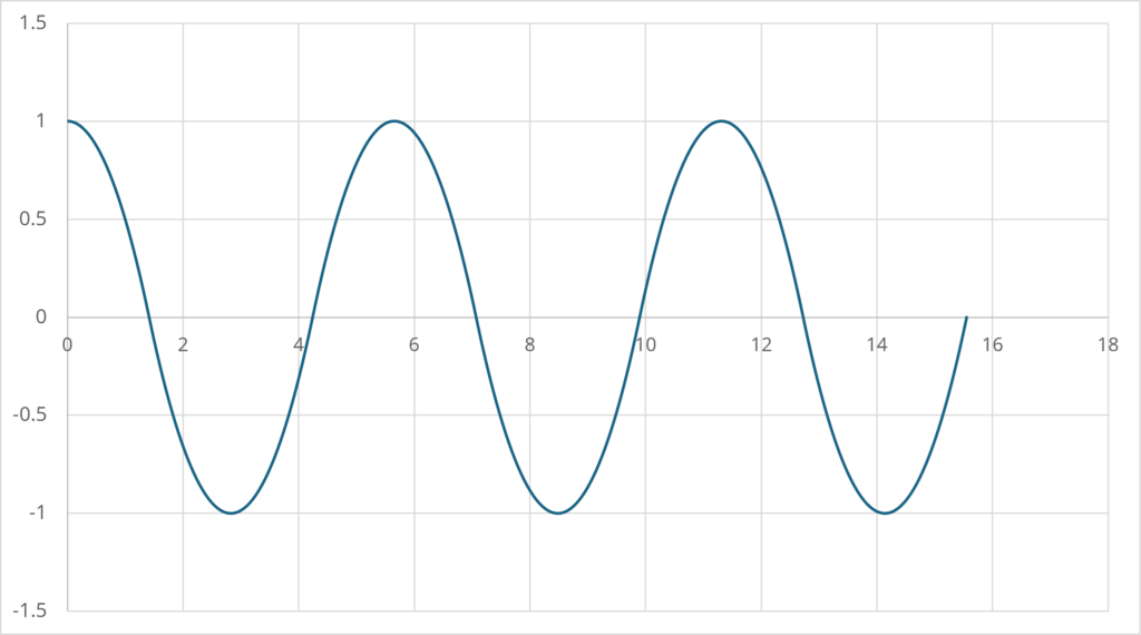
can be obtained. When graphed, it looks like this (calculated using \(\small x_0=1,g=1\)).
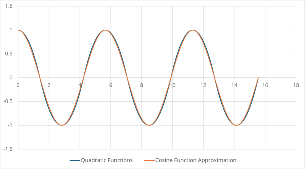
Note that while they may look like trigonometric functions, the individual functions that make up the period are quadratic, but can be approximated to a considerable degree by trigonometric functions. Specifically, if it has a maximum value \(\small x_0\) at time 0 and the period is \(\small T\), it can be approximated as:
\[ \small x(t) = x_0\cos\frac{2\pi t}{T}=x_0\cos \frac{\pi}{2\sqrt{2}}\sqrt{\frac{g}{x_0}}t. \]
Note that the period \(\small T\) can be calculated as:
\[ \small T = 4\sqrt{\frac{2x_0}{g}}. \]
In the above example, it is
\[ \small x(t) = \cos\frac{\pi}{2\sqrt{2}}t. \]
The actual comparison is as follows:
Of course, if the mass at the origin had a spatial dimension and the moving object landed there, it would remain at the origin. If not, gravity is presumably the force that causes periodic motion.
Two-body Problem in One-dimensional Space
I have derived the equation of motion for gravity in one dimension, but it still seems that fixing one of the mass points at the origin is not appropriate. Although the relative motion of two masses is as described above, each mass should be described as having its own independent motion. If we define the potential function as a two-body problem, it may be:
\[ \small V = -Gm_1m_2|x_1-x_2|. \]
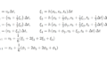
In this case, the acceleration of each mass can be calculated as:
\[ \small \begin{align*} &\frac{d^2x_1}{dt^2} = -Gm_2\text{sign}(x_1-x_2) \\ &\frac{d^2x_2}{dt^2} = -Gm_1\text{sign}(x_2-x_1). \end{align*} \]
Careful calculation will show that
\[ \small V=m_1x_1\frac{d^2x_1}{dt^2}+m_2x_2\frac{d^2x_2}{dt^2}=-Gm_1m_2|x_1-x_2| \]
holds true. Since four integration constants are required, four boundary conditions must be defined. Since making it too general would make the calculations more tedious, let us assume that it is given by
\[ \small x_1(0) = \frac{x_0}{2},\; x_2(0) = -\frac{x_0}{2},\; \frac{dx_1(0)}{dt} = 0,\; \frac{dx_2(0)}{dt} = 0. \]
Without loss of generality, let us assume that \(\small x_0>0\) and specify the equation of motion in this case.
At the initial point in time, \(\small x_1(t)>x_2(t)\), so the acceleration is:
\[ \small \begin{align*} &\frac{d^2x_1}{dt^2} = -Gm_2 \\ &\frac{d^2x_2}{dt^2} = Gm_1, \end{align*} \]
and we can find the solution by integrating each equation. If we calculate naively, we can obtain
\[ \small \begin{align*} &\frac{dx_1}{dt} = -Gm_2t \\ &\frac{dx_2}{dt} = Gm_1t, \end{align*} \]
and
\[ \small \begin{align*} &x_1(t) = \frac{x_0}{2}-\frac{1}{2}Gm_2t^2 \\ &x_2(t) = -\frac{x_0}{2}+\frac{1}{2}Gm_1t^2. \ \end{align*} \]
Find \(\small t\) when \(\small x_1(t)=x_2(t)\) occurs, we get
\[ \small -\frac{1}{2}G(m_1+m_2)t^2+x_0 = 0, \]
hence,
\[ \small t = \pm\sqrt{\frac{2x_0}{G(m_1+m_2)}}\]
can be obtained. \(\small t\) takes a positive value. Therefore,
\[ \small \begin{align*} &x_1(t) = \frac{x_0}{2}-\frac{1}{2}Gm_2t^2, \quad t \in \left[0, \sqrt{\frac{2x_0}{G(m_1+m_2)}}\right] \\ &x_2(t) = -\frac{x_0}{2}+\frac{1}{2}Gm_1t^2, \quad t \in \left[0, \sqrt{\frac{2x_0}{G(m_1+m_2)}}\right] \end{align*} \]
can be obtained. The velocity is:
\[ \small \begin{align*} &\frac{dx_1(t)}{dt}\Biggl|_{t=\sqrt{2x_0/G(m_1+m_2)}} = -Gm_2t = -m_2\sqrt{\frac{2x_0G}{m_1+m_2}} \\ &\frac{dx_2(t)}{dt}\Biggl|_{t=\sqrt{2x_0/G(m_1+m_2)}} = Gm_1t = m_1\sqrt{\frac{2x_0G}{m_1+m_2}}
\end{align*} \]
when \(\small x_1(t)=x_2(t)\).
As in the previous section, if we calculate the equation of motion for the interval \(\small x_1(t)<x_2(t)\), the velocity can be calculated as;
\[ \small \begin{align*} &\frac{dx_1}{dt} = Gm_2t-2m_2\sqrt{\frac{2x_0G}{m_1+m_2}} \\ &\frac{dx_2}{dt} = -Gm_1t+2m_1\sqrt{\frac{2x_0G}{m_1+m_2}}, \end{align*} \]
and the coordinates are
\[ \small \begin{align*} &x_1(t) =\left(\frac{1}{2}+\frac{2m_2}{m_1+m_2}\right)x_0-2tm_2\sqrt{\frac{2x_0G}{m_1+m_2}}+\frac{1}{2}Gm_2t^2 \\ &x_2(t) =-\left(\frac{1}{2}+\frac{2m_1}{m_1+m_2}\right)x_0+2tm_1\sqrt{\frac{2x_0G}{m_1+m_2}}-\frac{1}{2}Gm_1t^2. \end{align*} \]
\(\small t\) when \(\small x_1(t)=x_2(t)\) occurs can be calculated as:
\[ \small \begin{align*} &3x_0-2t(m_1+m_2)\sqrt{\frac{2x_0G}{m_1+m_2}}+\frac{1}{2}G(m_1+m_2)t^2=0 \\ \Rightarrow &t = 2\sqrt{\frac{2x_0}{G(m_1+m_2)}}\pm\sqrt{\frac{2x_0}{G(m_1+m_2)}}. \end{align*} \]
From the above, we can infer that the equation switches in period:
\[ \small 2\sqrt{\frac{2x_0}{G(m_1+m_2)}}. \]
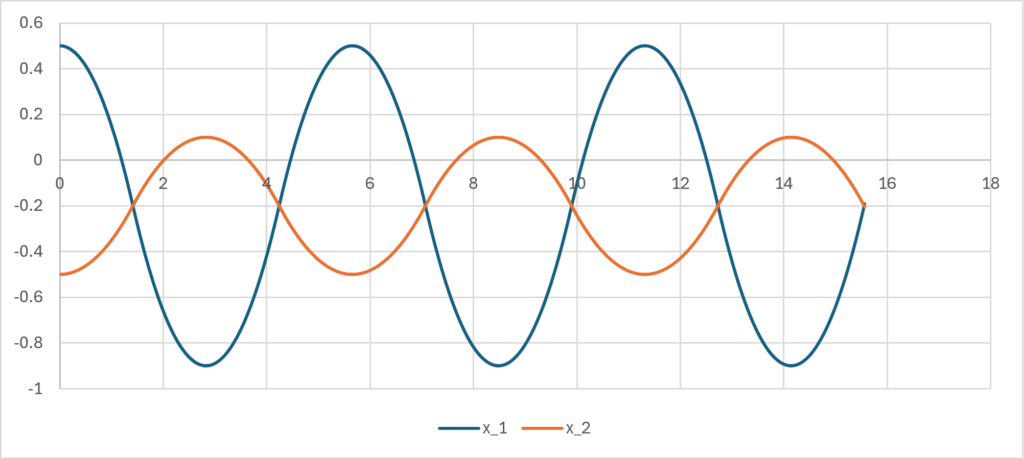
If we calculate this as in the previous section and connect the graph, we get the following (in the case of \(\small m_1=m_2=1/2\)).
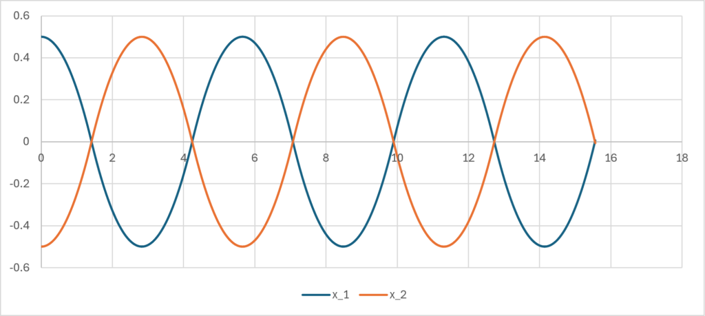
Note that in this solution, \(\small x_1(t)-x_2(t)\) is the same as \(\small x(t)\) in the previous section. In fact, as long as \(\small m_1+m_2=1\), the path \(\small x_1(t)-x_2(t)\) is the same function. For example, if \(\small m_1=0.3,m_2=0.7\), the respective paths are as follows, but the difference is the same as the result in the previous section.
In other words, the path of motion over distance caused by gravity depends only on the sum of the masses \(\small m_1+m_2\), and the proportions of the masses do not affect it. When approximated by trigonometric functions, it can be approximated as:
\[ \small \begin{align*} &x_1(t) = \frac{x_0}{2}+x_0\frac{m_2}{m_1+m_2}\left[\cos \frac{\pi t}{2\sqrt{2}}\sqrt{\frac{G(m_1+m_2)}{x_0}}-1\right] \\ &x_2(t) = -\frac{x_0}{2}-x_0\frac{m_1}{m_1+m_2}\left[\cos \frac{\pi t}{2\sqrt{2}}\sqrt{\frac{G(m_1+m_2)}{x_0}}-1\right]. \end{align*} \]
By the way, you may think that the graph shown above was calculated by solving the equations properly, but it is actually a graph that was solved numerically using the Runge-Kutta method. Well, in this age of advanced computers, there is no need to solve equations seriously…
Summary and Further Direction
The content discussed in this article is solely about motion when considering gravity in Euclidean space, and it will be necessary to extend this to relativistic space-time (conical coordinate system). In the general theory of relativity, gravity is considered to be a force that curves space-time, but I would like to consider what influence this concept has in a conical coordinate system (where space is spherical and therefore curved from the start). It’s easier to visualize and draw specific graphs if you think about it in one dimension rather than three, so I’ll try to think about this in the near future.
The problem we want to consider is how to deal with the motion of two substances in one coordinate system, when the motion of the two substances is represented by
\[ \small \begin{align*} &x_1^2+c^2T_{x_1,t}^2 = c^2t^2 \\
&x_2^2+c^2T_{x_2,t}^2 = c^2t^2. \end{align*} \]
This is probably illogical, but we must combine two 3-spheres so that the sum of the two 3-spheres is again a 3-sphere. This is due to the need to satisfy the relativistic property that the sum of the speeds of two lights moving at the speed of light must also be the speed of light. The question is what would happen if we considered the same thing with matter that has mass, that is, matter that moves slower than the speed of light, and the nature of this composition rule may be related to the essence of gravity. For example, if it is something like
\[ \small \begin{align*} &E_1^2 = m_1^2c^4+p_1^2c^2 \\ &E_2^2 = m_2^2c^4+p_2^2c^2 \\ &E^2 = (E_1+E_2)^2-2E_1E_2(E_1+E_2)G\frac{|r|}{c^4} \\ &\quad\;\; = E_1^2+E_2^2+2E_1E_2\left(1-\frac{G(E_1+E_2)|r|}{c^4}\right), \end{align*} \]
then it becomes
\[ \small E \approx E_1+E_2-G\frac{E_1}{c^2}\frac{E_2}{c^2}|r|, \]
and we may be able to provide a certain degree of justification for the classical mechanical approximation. The author believes that the shape of the formula leads to the hypothesis that
\[ \small \rho = 1-\frac{G(E_1+E_2)|r|}{c^4}, \]
in three-dimensional space
\[ \small \rho =1-\frac{G(E_1+E_2)}{c^4r}, \]
may represent some kind of correlation coefficient. This would mean that \(\small \rho \leq 0\) corresponds to the black hole solution in the Schwarzschild solution. The summation of energy on a sphere may be similar to calculating the variance in the summation of random variables.
In addition, we have considered the dimension of space in one dimension, but if we expand this to include what happens if it becomes two-dimensional, or what happens if it becomes three-dimensional, we may be able to arrive at the essence of gravity. Of course, we may not be able to understand the mechanism by which gravity is generated, but we may be able to find meaning in the fact that it may enable us to avoid the acrobatic interpretations of general relativity, such as distorting space (perhaps we may be able to reduce the effects of gravity to the nature of time).

Comments