
Problem Formulation
Consider a one-dimensional Coulomb potential:
\[ \small E = \frac{p^2}{2m}+e^2|x|. \]
In the one-dimensional case, it is not actually clear what the potential function is, but let us assume that it is
\[ \small V(r) = -\frac{e^2}{r^{D-2}} \]
when the dimension is \(\small D\) (For \(\small D = 1\) , the sign is reversed.). The fact that the one-dimensional Coulomb potential is a function proportional to the coordinate difference has been given some support, for example by Dirac (1932) (it seems that it involves a coefficient of \(\small 2\pi\), but we will omit this here). Let us find a solution to the Schrödinger equation:
\[ \small i\hbar\frac{\partial\psi(x,t)}{\partial t} = -\frac{\hbar^2}{2m}\frac{\partial^2\psi(x,t)}{\partial x^2}+e^2|x|\psi(x,t) \]
derived from the correspondence principle in quantum mechanics. Since it is difficult to solve this type of equation directly, we will consider
\[ \small \begin{align*} &i\hbar\frac{\partial\psi(x,t)}{\partial t} = -\frac{\hbar^2}{2m}\frac{\partial^2\psi(x,t)}{\partial x^2}+e^2x\psi(x,t), \quad x>0 \\
&i\hbar\frac{\partial\psi(x,t)}{\partial t} = -\frac{\hbar^2}{2m}\frac{\partial^2\psi(x,t)}{\partial x^2}-e^2x\psi(x,t), \quad x<0 \end{align*} \]
by dividing the region into \(\small x>0\) and \(\small x<0\), just like one-dimensional gravity. This problem is often called the triangular well potential problem, and it seems to be solved using the Airy function. However, since it is difficult to imagine a specific probability distribution even if we find the basis functions, we will try to guess the form of the solution using a simple approximation.
Assume that \(\small x>0\) at \(\small t=0\), and let the expected value of the coordinate and the momentum at that time be \(\small x_0,p_0\). As an approximation, we assume that the uncertainty in the coordinates follows a normal distribution and that the wave function at the initial time is:
\[ \small \psi(x, 0) = \psi(x,0) = \frac{1}{\sigma^{1/2}\pi^{1/4}} \exp\left(-\frac{(x-x_0)^2}{2\sigma^2}\right) \exp \left( \frac{i}{\hbar} p_0 (x-x_0) \right). \]
This is an approximation because it has a probability even for \(\small x<0\). We assume that \(\small \sigma\) is small enough that such a probability can be ignored. From the above, the basic equation and boundary condition of the problem to be solved are:
\[ \small \begin{align*} &i\hbar\frac{\partial\psi(x,t)}{\partial t} = -\frac{\hbar^2}{2m}\frac{\partial^2\psi(x,t)}{\partial x^2}+e^2x\psi(x,t), \quad x > 0 \\ &\psi(x,0) = \frac{1}{\sigma^{1/2}\pi^{1/4}} \exp\left(-\frac{(x-x_0)^2}{2\sigma^2}\right) \exp \left( \frac{i}{\hbar} p_0 (x-x_0) \right), \end{align*} \]
and we need to find \(\small \psi(x,t)\) in this case. Although it’s a bit of a cheaty method, let us try to find an approximate solution.
Deriving an Approximate Solution
The boundary condition is Fourier transformed and set as:
\[ \small \psi(x,0) = \int_{-\infty}^\infty A_k\exp(ikx) dk. \]
When the amplitude is calculated from the inverse Fourier transform, it was
\[ \small A_k = \frac{\sigma}{\sqrt{2\pi}}\frac{1}{\sigma^{1/2}\pi^{1/4}}\exp\left(-\frac{\sigma^2}{2}\left(\frac{p_0}{\hbar}-k\right)^2\right). \]
Assume \(\small \psi_k(x, t) = A_k\exp(ikx-i\omega t)\) and since
\[ \small \frac{\partial \psi_k(x,t)}{\partial x} = ik\psi_k(x,t), \]
we get
\[ \small \frac{\partial^2 \psi_k(x,t)}{\partial x^2} = -k^2\psi_k(x,t). \]
Substituting into the Schrödinger equation,
\[ \small \frac{\partial \psi_k(x,t)}{\partial t} = -\left(i\frac{\hbar k^2}{2m}-i\frac{e^2}{\hbar}x\right)\psi_k(x,t) \]
can be obtained. Since
\[ \small \frac{\partial \ln \psi_k(x,t)}{\partial t} = \frac{1}{\psi_k(x,t)}\frac{\partial \psi_k(x,t)}{\partial t}, \]
by integrating with respect to time,
\[ \small \ln \psi_k(x,t) = -i\frac{\hbar k^2}{2m}t+i\frac{e^2}{\hbar}\int_0^tx(u)du+C \]
can be obtained. By defining the integral constant \(\small C\) so that the boundary condition is satisfied when \(\small t=0\), we get
\[ \small \psi_k(x,t) = \exp\left(ik(x-x_0)-i\frac{\hbar k^2}{2m}t+i\frac{e^2}{\hbar}\int_0^tx(u)du \right) \]
(The signs seem to be reversed, but I’ll ignore that.).
The question arises as to how to define the integral of \(\small x\) with respect to time, but based on classical mechanical approximations, we can infer that on average it is:
\[ \small x(u) \approx x_0+\frac{p_0}{m}u-\frac{1}{2}\frac{e^2}{m}u^2. \]
Acceleration is calculated using \(\small ma=-e^2\). If we calculate the integral,
\[ \small \int_0^tx(u)du = x_0t+\frac{p_0}{2m}t^2-\frac{1}{6}\frac{e^2}{m}t^3 \]
can be obtained. By substituting this into the basis functions of the wave function, it can be expressed as:
\[ \small \psi_k(x,t) = \exp\left(ik(x-x_0)-i\frac{\hbar k^2}{2m}t+i\frac{e^2}{\hbar}x_0t+ik\frac{e^2}{2m}t^2-i\frac{e^4}{6m\hbar}t^3 \right). \]
Therefore, the wave function can be calculated as:
\[ \small \begin{align*} \psi(x,t) = & \frac{\sigma}{\sqrt{2\pi}}\frac{1}{\sigma^{1/2}\pi^{1/4}} \\ & \times \int_{-\infty}^\infty \exp\left(-\frac{\sigma^2}{2}\left(\frac{\bar{p}}{\hbar}-k\right)^2+ik(x-x_0)-i\frac{\hbar k^2}{2m}t+i\frac{e^2}{\hbar}x_0t+ik\frac{e^2}{2m}t^2-i\frac{e^4}{6m\hbar}t^3 \right) dk. \end{align*} \]
It may seem complicated, but in fact, in the free particle solution:
\[ \small \begin{align*} \psi(x,t) \; & = \frac{1}{\pi^{1/4}\sigma^{1/2}} \frac{1}{\left( 1+\frac{i \hbar t}{m\sigma^2} \right)^{1/2}} \small \exp \left(- \frac{\left( x-\frac{\bar{p}}{m}t \right)^2}{2 \sigma^2 \left(1 + \left(\frac{\hbar t}{m\sigma^2} \right)^2 \right)} \right) \\ &\small \quad\;\times \exp \left(i \left\{ \frac{\bar{p}}{\hbar}x – \frac{\bar{p}^2 t}{2m \hbar} + \frac{\hbar t \left( x-\frac{\bar{p}}{m}t \right)^2}{2 m \sigma^4 \left(1 + \left( \frac{\hbar t}{m\sigma^2} \right)^2 \right)} \right\} \right), \end{align*} \]
if you replace \(\small x\) with \(\small x-x_0+e^2t^2/2m\) and multiply it by
\[ \small \exp\left(i\frac{e^2}{\hbar}x_0t-i\frac{e^4}{6m\hbar}t^3\right) \]
you can confirm that you will get the solution. This is because these term does not depend on \(\small k\) and can therefore be taken out of the integral. In summary, we can get
\[ \small \begin{align*} \psi(x,t) \; & = \frac{1}{\pi^{1/4}\sigma^{1/2}} \frac{1}{\left( 1+\frac{i \hbar t}{m\sigma^2} \right)^{1/2}} \small \exp \left(- \frac{\left( x-x_0-\frac{p_0}{m}t +\frac{1}{2}\frac{e^2}{m}t^2\right)^2}{2 \sigma^2 \left(1 + \left(\frac{\hbar t}{m\sigma^2} \right)^2 \right)} \right) \\ &\small \quad\;\times \exp \left(i \left\{ \frac{p_0}{\hbar}x – \frac{p_0^2 t}{2m \hbar}+\frac{e^2}{\hbar}x_0t +\frac{p_0e^2}{2m\hbar}t^2-\frac{e^4}{6m\hbar}t^3+ \frac{\hbar t \left( x-x_0-\frac{p_0}{m}t+\frac{1}{2}\frac{e^2}{m}t^2 \right)^2}{2 m \sigma^4 \left(1 + \left( \frac{\hbar t}{m\sigma^2} \right)^2 \right)} \right\} \right). \end{align*} \]
The partial differential equation that this solution satisfies is:
\[ \small i\hbar\frac{\partial\psi(x,t)}{\partial t} = -\frac{\hbar^2}{2m}\frac{\partial^2\psi(x,t)}{\partial x^2}+e^2\left(x_0+\frac{p_0}{m}t-\frac{1}{2}\frac{e^2}{m}t^2 \right)\psi(x,t), \]
which is different from the original fundamental equation, but if you replace it with
\[ \small x = x_0+\frac{p_0}{m}t-\frac{1}{2}\frac{e^2}{m}t^2, \]
you can confirm that the two are approximately the same. When \(\small x<0\), the sign of the acceleration term is simply reversed.
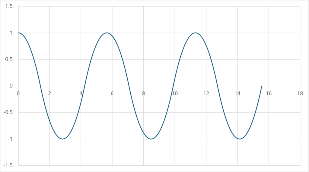
From the above, we can infer that the motion of an electron bound to a one-dimensional Coulomb potential is the motion obtained by adding a quantum mechanical uncertainty term to the periodic motion considered in one-dimensional gravity (the graph below to which normal distribution noise has been added).
Is the steady state just a fiction?
Perhaps some readers who have read this far will think that instead of such an approximate solution, I should calculate the probability distribution in the steady state (a solution that does not depend on \(\small t\)). However, in reality, quantum phenomena are thought to be probabilistic, and it can be assumed that each point in time does not strictly have the same detection probability distribution. The probability distribution changes over short time intervals, but because the time intervals are so short, we are under the illusion that the probability distribution is steady (does not change over time). One might think that unless it is a steady state, it will not be a stable state, but with a periodic solution such as the one above, it is thought that the movement will have a certain degree of stability even if it is not steady. When we think about it this way, it is important to note that the steady-state solution is a model that we humans think of, and that real quantum may not be in such a state.
For example, consider the case in which the periodic motion in the above example is so fast that it is impossible to distinguish at which point in one period it is detected. In that case, this means that it is impossible to determine at what point \(\small t\) it will be detected for \(\small x(t)\) that satisfies
\[ \small \begin{align*} &x(t)=a-\frac{1}{2}\frac{e^2}{m}t^2, \quad x\in[0,a] \\ &x(t)=-a+\frac{1}{2}\frac{e^2}{m}t^2, \quad x\in[-a, 0]. \end{align*} \]
If we assume that \(\small t\) is a uniformly distributed random variable, then its domain is:
\[ \small t \in \left[0, \sqrt{\frac{2ma}{e^2}}\right], \]
and therefore the probability density function of \(\small t\) is:
\[ \small p(t) = \sqrt{\frac{e^2}{2ma}}. \]
Since the inverse function of \(\small x(t)\) is:
\[ \small t(x) = \sqrt{\frac{2m}{e^2}(a-x)}, \]
the probability density function of \(\small x(t)\) for \(\small x>0\) can be calculated as:
\[ \small p(x) = \frac{\sqrt{\frac{e^2}{2ma}}\frac{dt(x)}{dx}}{\int_0^a\sqrt{\frac{e^2}{2ma}}\frac{dt(x)}{dx}dx} = \frac{1}{2\sqrt{a(a-x)}}, \quad x \in[0,a]. \]
Since the probability distribution is symmetric between \(\small x>0\) and \(\small x<0\),
\[ \small p(x) = \frac{1}{4\sqrt{a(a-|x|)}}, \quad x \in [-a,a] \]
will be the probability density function. The probability distribution obtained by adding quantum mechanical noise to this may be the probability distribution in the steady state. However, this probability distribution would probably be difficult to derive from a wave function that satisfies the Schrödinger equation for a one-dimensional Coulomb potential. In other words, there may be cases where the solution of the steady-state Schrödinger equation does not adequately derive the detection probability distribution of the electron. In order to derive an appropriate detection probability distribution, it may be necessary to solve the time-dependent Schrödinger equation and then calculate the time-averaged probability distribution as described above.
Appendix: Airy Functions
The Airy functions are functions defined by
\[ \small \begin{align*} &\text{Ai}(x) = \frac{1}{\pi}\int_0^\infty \cos\left(\frac{t^3}{3}+xt \right)dt \\ &\text{Bi}(x) = \frac{1}{\pi}\int_0^\infty \exp\left(-\frac{t^3}{3}+xt \right)+\sin\left(\frac{t^3}{3}+xt \right)dt, \end{align*} \]
which are the solutions to the differential equation:
\[ \small \frac{d^2f(x)}{d^2x}-xf(x) =0. \]
The solution of the Schrödinger equation:
\[ \small i\hbar\frac{\partial\psi(x,t)}{\partial t} = -\frac{\hbar^2}{2m}\frac{\partial^2\psi(x,t)}{\partial x^2}+e^2x\psi(x,t) \]
for the one-dimensional Coulomb potential can be expressed as:
\[ \small E\Psi(x) =-\frac{\hbar^2}{2m}\frac{d^2\Psi(x)}{dx^2}+e^2x\Psi(x) \]
by placing
\[ \small \psi(x,t) = \Psi(x)\exp\left(-i\frac{E}{\hbar}t \right) \]
as the solution. Hence, the equation can be transform to
\[ \small \frac{d^2\Psi(x)}{dx^2} + \frac{2me^2}{\hbar^2}\left(\frac{E}{e^2}-x\right)\Psi(x)=0. \]
If we change the variables to
\[ \small \xi =-\left(\frac{E}{e^2}-x \right)\left(\frac{\hbar^2}{2me^2}\right)^{-\frac{1}{3}}, \]
we get
\[ \small \frac{d^2\Psi(\xi)}{d\xi^2}-\xi\Psi(\xi)=0, \]
and the differential equation for the Airy function can be obtained. Therefore, the solution can be found in the form of
\[ \small \Psi(\xi) = c_1\text{Ai}(\xi)+c_2\text{Bi}(\xi), \]
and the wave function can be expressed as a linear combination of functions based on the Airy functions. However, the value of the energy must be solved as an eigenvalue problem, and it is probably not possible to derive the wave function analytically.
It may seem that there is no relationship between the approximate solution derived in this article and the Airy functions. However, it seems that if we consider the Taylor expansion of the Hermite polynomial of three variables, it can be expressed as:
\[ \small \exp\left(xt+yt^2+zt^3 \right) = \sum_{n=0}^\infty {}_3H_n(x,y,z) \frac{t^n}{n!}. \]
It seems that this Hermite polynomial of three variables can be expressed as:
\[ \small {}_3 H_n(x,y,z) = \int_{-\infty}^\infty \xi^n\text{GAi}(\xi-x,y,z)d\xi \]
using the Gauss-Airy function:
\[ \small \text{GAi}(x,y,z) = \frac{1}{\pi}\int_0^\infty e^{-yt^2}\cos\left(xt-zt^3\right)dt \]
(The symbols are confusing, but \(\small y,z\) can be constants. If you set \(\small y=0,z=-1/3\), you can see that it becomes an Airy function.). It seems that if we can transform the equation properly, we can bring it into this form and give a certain degree of validity to the calculations in this article, which use a cubic function with respect to \(\small t\)…but that seems impossible, so I’ll stop here.
Reference
[1] Dirac, Paul.A.M (1932), Relativistic Quantum Mechanics. Proceedings of the Royal Society A, 136, 453-464.


Comments