Problem Formulation
Let us consider a way to maximize the profit obtained by repeating a gamble of choosing one option from options with expected value \(\small \mu_1,\cdots,\mu_n\) a fixed number of times \(\small T\). However, unlike general problems, we assume that the gambler does not know in advance the true expected value of each choice \(\small \mu_1,\cdots,\mu_n\). Therefore, in order to estimate the expected value, it is necessary to use information obtained through a certain number of trials. Unlike decision-making problems where the probability distribution is known in advance, decision-making problems where the probability distribution is unknown in advance are called incomplete information problems. This problem is a type of optimization problem that deals with the trade-off between the opportunity to explore information (Exploration) and the opportunity to utilize the obtained information to make a profit (Exploitation), and is known as the multi-armed bandit problem.
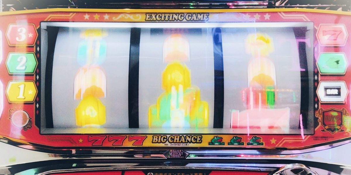
A type of gambling that is often cited as an example of the multi-armed bandit problem is slot machines (pachinko in Japan; by the way, pachinko is almost exclusively a Japanese culture and is either banned or barely popular overseas). This involves making a decision to explore which machines have a higher expected value and then continuing to play the machines with the higher expected value that you discover in order to earn more profits. In reality, many games of imperfect information can be formulated as multi-armed bandit problems, and Texas Hold’em may be an equivalent mathematical problem in that it involves exploring which arm to draw on a slot machine – raise, call, or fold – to maximize the expected value, and then exploiting the information obtained.
I don’t know much about it, but it seems that seriously trying to estimate the expected value of Japanese pachinko is a fairly difficult mathematical problem. It might be easy if all we needed to know was the probability of winning or the average number of balls paid out, but it seems that there are some events whose probabilities fluctuate (and need to be modeled as stochastic processes), and this needs to be taken into account when calculating the expected value. What this means is that we need to make a Bayesian estimate of the expected value of the machine from the observed values of these various events. If you think about it this way, the fun of Texas Hold’em may be similar to that of pachinko (slot machines). Well, if someone told you that “pachinko is an intellectual mathematical game,” you might laugh…Maybe the idea that “Texas Hold’em is an intellectual mind sport!” has the same vibe? Well, I’ll think about applications to Texas Hold’em later, but the purpose of this article is to give an overview of the multi-armed bandit problem without going into complex proofs or calculations.
Stochastic Optimization Problems under Incomplete Information and Minimizing Expected Regret
Suppose there are \(\small n\) slot machines with expected values \(\small \mu_1, \cdots, \mu_n \), and we know the expected value of each machine from the beginning. In this case, the optimization problem is a complete information problem, and the optimal action is to play the machine with the highest expected value \(\small T\) times. If \(\small u_i(t)\) is the revenue observed at the machine of \(\small i\), then the expected revenue obtained at this time is given by
\[ \small P_\sigma(T) = E\left[\sum_{t=1}^T u_{\sigma(t)}(t)\right]=\mu^{\ast} T, \quad \mu^\ast=\max\{\mu_1,\cdots,\mu_n\}. \]
This can be seen as the result of determining the optimal policy \(\small \sigma\) to be
\[ \small \max_{\sigma} E\left[\sum_{t=1}^T u_{\sigma(t)}(t)\right]. \]
Even if the calculation of the expected value is complicated, it will generally be possible to calculate this expected value by constructing a model and performing a Monte Carlo simulation.
In reality, the expected value of each machine is unknown, so let
\[ \small \hat{Q}_{\pi}(T) = \sum_{t=1}^T u_{\pi(t)} \]
denote the revenue when selecting a machine according to some policy \(\small \pi\). \(\small \hat{Q}(T)\) would be the revenue obtained as a solution to the incomplete information problem. Even in stochastic optimization problems under incomplete information, such as the multi-armed bandit problem, one might think that it is sufficient to simply determine the optimal policy \(\small \pi\) so that
\[ \small \max_{\pi} Q_{\pi}(T) = E[\hat{Q}_{\pi}(T)]= \sum_{t=1}^T \mu_{\pi(t)} \]
is the solution.
However, unlike the complete information problem, with incomplete information the expected value of each machine is unknown, so it is not possible to simulate the revenue of each machine in advance and estimate \(\small Q_{\pi}(T)\). This means that the expected profit for each machine is not known until the machine is actually played, and it is not possible to perform a Monte Carlo simulation in advance to determine the optimal strategy. Therefore, it is necessary to determine the optimal course of action based on information obtained after the fact. The revenue observed for each machine at the \(\small t\)-th time (ex post observation) is denoted as \(\small u_1(t),\cdots,u_n(t)\), and the ex post average revenue is denoted as:
\[ \small \hat{\mu}_i = \frac{1}{T}\sum_{t=1}^T u_i(t). \]
In this case, if we determine the optimal strategy as a complete information problem based on ex-post information, the optimal solution will be to play the machine with the highest ex-post average profit \(\small T\) times, so the answer is:
\[ \small \hat{P}_\sigma(T) = \sum_{t=1}^T u_{\sigma(t)}(t)=\hat{\mu}^{\ast} T, \quad \mu^\ast=\max\{\hat{\mu}_1,\cdots,\hat{\mu}_n\}. \]
The difference:
\[ \small R(T) =\hat{P}_\sigma(T)-\hat{Q}_{\pi}(T) \]
between the payoff \(\small \hat{P}_{\sigma}(T)\) obtained from the optimal policy for the complete information problem based on this ex-post information and the payoff \(\small \hat{Q}_{\pi}(T)\) in the incomplete information problem when playing the game according to the policy \(\small \pi\) is called regret. In an incomplete information problem, it is necessary to determine the optimal policy \(\small \pi^\ast \) that minimizes the expected value:
\[ \small E[R(T)] =\hat{\mu}^{\ast} T -\sum_{t=1}^T \hat{\mu}_{\pi(t)} \]
of the regret.
From the definition of regret, it is easy to see that in a complete information problem, if one plays the game according to the optimal policy \(\small \sigma^\ast\), the expected regret will be 0. In incomplete information problems, it is generally true that \(\small E[R(T)]>0\), and the magnitude of this value corresponds to the cost of having incomplete information. The optimal strategy would be one that balances the trade-off between the search costs of obtaining this information and the actions required to obtain benefits based on the information obtained, in the optimal ratio. By the way, the difference between the mathematical problems known as Reinforcement Learning in machine learning and artificial intelligence problems and general stochastic dynamic optimization problems is whether the information is incomplete or complete, and it should be noted that the mathematical problems that Reinforcement Learning targets are stochastic dynamic optimization problems under incomplete information.
Examples of Solution Algorithm
We will introduce some well-known algorithms for solving multi-armed bandit problems. We will briefly explain three methods: the ε-greedy method, the UCB method, and the probability matching method.
1. ε-greedy Method
The ε-greedy method is a solution method that assigns a certain proportion of the possible trials \(\small T\) (\(\small 0 < \epsilon < 1\), \(\small \epsilon T\)) to a search to estimate the expected value of each machine, and then assigns the machine with the highest expected value among the estimated expected values to be tried for the remaining \(\small (1-\epsilon)T\) trials. There are variations in the search behavior used to estimate a machine’s expected value, but typically it is sufficient to draw all options equally and estimate
\[ \small \hat{\mu_i} = \frac{n}{\epsilon T}\sum_{t=(i-1)\epsilon T/n}^{i\epsilon T/n} u_i(t). \]
\(\small \epsilon\) is a hyperparameter and an appropriate value must be given exogenously.
2. UCB Method
The ε-greedy method searches all machines equally regardless of the observed average value, which may result in large search costs (losses). Therefore, it may be possible to reduce search costs by exploring less machines with low observed profits and exploring more machines with high profits. On the other hand, there is a disadvantage in that a smaller number of trials results in a worsening accuracy in estimating the expected value of that machine. One way to strike this balance is to estimate the expected value of each machine as:
\[ \small \hat{\mu}_i(\tau) =\frac{1}{N_i(\tau)}\sum_{t=1}^{\tau} 1_{\{\pi(t)=i\}}u_{\pi(t)}(t)+\sqrt{\frac{\log \tau}{2N_i(\tau)}} \]
and in the \(\small t\)-th time, choose the option with the highest \(\small \hat{\mu}_i(t)\). Here, \(\small N_i(\tau)\) represents the number of times option \(\small i\) was chosen in the \(\small \tau\)-th iteration. This increases the chances that an option that has been chosen less frequently will be chosen even if the observed profit is low. The formula itself seems to be calculated on the assumption that the profit follows a Bernoulli distribution.
3. Probability Matching Method
Like the mixed strategy in game theory, this method calculates the probability distribution of choosing option \(\small i\) using a multinomial logit model:
\[ \small p_i = \frac{e^{f(\hat{\mu}_i)}}{\sum_{i=1}^n e^{f(\hat{\mu}_i)}}, \]
and then selects an option randomly according to that probability distribution. The score \(\small s=f(\hat{\mu}_i)\), which is the weight of which option should be chosen, needs to be determined from the prior prediction (prior distribution) of the probability distribution of the revenue for each option. This will be estimated using Bayesian estimation (where a prior distribution is determined based on the gambler’s beliefs and parameters are updated from observed values).
The most sophisticated method would be the probability matching method, but it seems to have some difficult aspects for a human to conceive and execute. In reality, the ε-greedy method is empirically easy to handle, but the expected regret varies greatly depending on how \(\small \epsilon\) is set, so some experience or intuition may be needed to set an appropriate \(\small \epsilon\) depending on the problem.
Appendix: Why Pachinko Balls Don’t Move in the Same Trajectory
I have never played pachinko and do not know much about how it works, but what I find strange is why the pachinko balls, even though they are hit in the same way, take completely different, random trajectories. From a classical mechanics perspective, it seems likely that if the same force is applied to an object of the same mass, even a pachinko machine with many nails would move in the same trajectory. It seems that there is a random element in the initial conditions, which is amplified by the nails in the pachinko machine, resulting in chaotic random movement. The following factors seem to be random in the initial conditions:
- The mechanism that shoots out the pachinko balls is spring-loaded, and even if the lever is completely fixed, there is uncertainty as to the direction of the force and the rotation of the ball (random vibrations or rotations may be applied).
- Although pachinko balls all appear to be made with the same mass, it seems that subtle individual differences are intentionally created, which causes them to not move in the same trajectory even when the same force is applied to them.
- Because multiple pachinko balls are in the machine at the same time, multiple balls collide with each other, creating an element of randomness.
Due to these factors, it seems that it is basically impossible to increase your winning rate by changing the way you hit the pachinko lever.
Similarly, foreign slot machines also have three spinning reels that stop, but you might be wondering whether timing the action makes it easier to hit a jackpot. Unfortunately, this also seems to be impossible. In fact, when you pull the lever on a slot machine, a random number is determined by the machine or digital control, and the winning or losing outcome is already decided by the time the player stops the reels. The operation of stopping the reels is a production that makes it look as if the player is making the decision himself, and it seems to have the effect of making the player feel elated when they hit a win. In fact, it doesn’t seem to matter at all when you stop the reels, so if you want to play efficiently, it seems like you should stop them quickly.
It seems that operations that affect the outcome of gambling based on the player’s skill are called skill-based play. In both pachinko and slot machines, skill-based play is basically impossible, and there seem to be few factors other than treating them as a multi-armed bandit problem in which you choose which machine to play (in Japanese pachislot machines, there are some models that allow you to slightly affect the probability by pressing buttons in the correct order or timing it correctly). Since poker is a game played against other players, it is of course a form of gambling that involves skill, but I am not sure to what extent this involves it. Although it may seem like a battle of wits, it is possible that most of the game is just a game of luck. For example, if all players are using rational strategies (Nash equilibrium strategies), it will be impossible to explain the outcome of a game by factors other than luck. Even if such a situation is impossible in reality, if the players’ skill levels are similar, the game will become a game of luck.


Comments