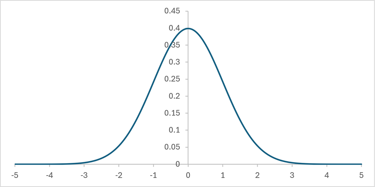
This article is a note on probability distribution. For two random numbers \(\small x,y \) that follow a normal distribution:
\[ \small \phi_{N(0,\sigma^2)}(x) = \frac{1}{\sqrt{2\pi\sigma^2}}\exp\left(-\frac{x^2}{2\sigma^2} \right), \]
the probability distribution that their sum, product, ratio, etc. follow is shown. We assume that the mean is 0 because if the mean is not 0, the calculations become complicated or it may not be possible to calculate it analytically at all. I would not provide a proof (although I may add one in the future).
Sum
Let assume \(\small x,y\sim N(0,\sigma^2)\). If there is no correlation, the probability distribution that \(\small z=x+y\) follows is normal, which is:
\[ \small z\sim N(0, 2\sigma^2). \]
If the correlation is \(\small \rho\), then it is:
\[ \small z \sim N(0, 2(1+\rho)\sigma^2). \]
For example, if the correlation is 1, it is:
\[ \small z \sim N(0, 4\sigma^2). \]
This can be found by defining \(\small z=x+y\) and calculating
\[ \small \phi(z) = \int_{-\infty}^\infty \phi_{N_2(0,0,\sigma^2,\sigma^2,\rho)}(z-y,y)dy \]
from the two-variable normal distribution function \(\small \phi_{N_2(0,0,\sigma^2,\sigma^2,\rho)}(x,y)\).
Generalizing and calculating for a sum of \(\small n\),
\[ \small \sum_{i=1}^n x_i\sim N(0,n\sigma^2) \]
holds when there is no correlation in \(\small x_1,\cdots,x_n\sim N(0,\sigma^2)\). Note that
\[ \small nx_1 \sim N(0, n^2\sigma^2) \]
holds. Multiplying a normal random number by \(\small n\) is equivalent to adding \(\small n\) random numbers with a correlation of 1, and it should be noted that adding \(\small n\) independent random variables and multiplying a normal random number by \(\small n\) have different probability distributions.
Product
Let assume \(\small x,y\sim N(0,\sigma^2)\). This can be found by defining \(\small z=xy\) and calculating
\[ \small \phi(z) = \int_{-\infty}^\infty\int_{-\infty}^\infty \delta\left(z-xy\right)\phi_{N_2(0,0,\sigma^2,\sigma^2,\rho)}(x,y)dxdy \]
from the two-variable normal distribution function \(\small \phi_{N_2(0,0,\sigma^2,\sigma^2,\rho)}(x,y)\). When \(\small \rho=0\), it seems that it can be calculated as:
\[ \begin{align*} & \small \phi(z) = \frac{1}{\pi\sigma} K_0\left(\frac{|z|}{\sigma} \right) \\ & \small K_0(x) = \int_0^\infty \frac{\exp\left(-t-\frac{x^2}{4t} \right)}{t} dt \end{align*} \]
using the modified Bessel function of the second kind \(\small K_\nu(x)\). The identity of the modified Bessel function of the second kind \(\small K_\nu(x)\) is unclear to the present author.
Another interesting thing is that if we define
\[ \small z = x_1x_4\pm x_2x_3 \]
for four independent standard normal random numbers \(\small x_1,x_2,x_3,x_4\sim N(0,1)\), then \(\small z\) follows the standard Laplace distribution:
\[ \small \phi_L(z) = \frac{1}{2}\exp(|z|). \]
This would correspond to the probability distribution of angular momentum:
\[ \small l_x = xp_y-yp_x \\ \small l_y = xp_x+yp_y \]
when coordinates \(\small x,y\) and momentum \(\small p_x,p_y\) follow independent normal distributions.
Ratio
Let assume \(\small x,y\sim N(0,\sigma^2)\). This can be found by defining \(\small z=x/y\) and calculating
\[ \small \phi(z) = \int_{-\infty}^\infty\int_{-\infty}^\infty \delta\left(z-\frac{x}{y} \right) \phi_{N_2(0,0,\sigma^2,\sigma^2,\rho)}(x,y)dxdy \]
from the two-variable normal distribution function \(\small \phi_{N_2(0,0,\sigma^2,\sigma^2,\rho)}(x,y)\). Assuming that \(\small \rho=0\), we get
\[ \small \phi_C(z) = \frac{1}{\pi}\frac{1}{1+z^2}, \]
which is the probability density function of a probability distribution called the Cauchy distribution.
Sum of Squares and Its Square Root
It is a common problem to find the probability distribution of
\[ \small x=\sum_{i=1}^n x_i^2 \]
when there is no correlation between \(\small x_1,\cdots,x_n\sim N(0,\sigma^2)\), and the resulting probability distribution is well known. This is a probability distribution called the \(\small \chi^2\) distribution (Chi-square Distribution), and the probability density function is calculated using the following function:
\[ \small \phi_{\chi^2(n, \sigma^2)}(x) = \frac{1}{2^{\frac{n}{2}}\Gamma\left(\frac{n}{2}\right)\sigma^{\frac{n}{2}}}x^{\frac{n}{2}-1}\exp\left(-\frac{x}{2\sigma}\right). \]
If you want to find the probability distribution of
\[ \small x =\frac{1}{n}\sum_{i=1}^n x_i^2 \]
for \(\small n\) uncorrelated standard normal random numbers \(\small x_1,\cdots,x_n\sim N(0,1)\), you can confirm that the probability distribution matches by replacing \(\small \sigma=1/n\) in the above equation.
Similarly, the probability distribution that the square root of the sum of squares:
\[ \small x=\sqrt{\sum_{i=1}^n x_i^2} \]
follows is often used, and is called the \(\small \chi\) distribution. Since the squared value of \(\small x\) follows the \(\small \chi^2\) distribution,
\[ \small \chi(x|n) = \chi^2(x^2|n) \]
holds true if we set \(\small \sigma=1\). Differentiating both sides with respect to \(\small x\) gives
\[ \small \phi_{\chi(n)}(x) = \frac{d(x^2)}{dx} \phi_{\chi^2(n)}(x^2)=2x\phi_{\chi^2(n)}(x^2). \]
By replacing \(\small x\) with \(\small x/\sigma\), we can obtain the probability density function for the \(\small \chi\) distribution. Therefore, the probability density function of the \(\small \chi \) distribution can be obtained as:
\[ \small \phi_{\chi(n,\sigma^2)}(x) = \frac{1}{2^{\frac{n}{2}-1}\Gamma\left(\frac{n}{2}\right)\sigma^n}x^{n-1}\exp\left(-\frac{x^2}{2\sigma^2}\right). \]
If you want to find the probability distribution of
\[ \small x =\sqrt{\frac{1}{n}\sum_{i=1}^n x_i^2} \]
for \(\small n\) uncorrelated standard normal random numbers \(\small x_1,\cdots,x_n\sim N(0,1)\), you can confirm that the probability distribution is the same by replacing \(\small \sigma=1/\sqrt{n}\) in the above equation.
General Probability Distribution of Ratios
Finally, let us extend the probability distribution of ratios to the case where the numerator and denominator are probability distributions other than normal (such as the \(\small \chi^2 \) distribution). For example, it is known that the ratio of a normal distribution and a \(\small \chi \) distribution results in a probability distribution called Student’s \(\small t\) distribution. This is a probability distribution that follows the standardized value obtained by dividing the probability distribution of the sample value by the sample standard deviation, and is a probability distribution that often appears in econometrics, etc. Another example is the probability distribution for the ratio of the variances of samples sampled from two normal distributions, which is the probability distribution for the ratio of random numbers sampled from two \(\small \chi^2 \) distributions, known as the \(\small F\) distribution.
As a generalization of these, we will show the probability distribution that the ratio value follows when the numerator and denominator follow the following probability distribution, which is called the generalized gamma distribution.
\[ \small \gamma(x|\sigma,n,d) = \frac{d}{\Gamma\left(\frac{n}{d}\right)\sigma^n}x^{n-1}\exp\left( -\left(\frac{x}{\sigma}\right)^d\right) \]
It can be understood that the generalized gamma distribution is a fairly generalized probability distribution that includes the normal distribution, the \(\small \chi^2 \) distribution, and the \(\small \chi \) distribution. If we assume that \(\small x,y\) follow the generalized gamma distributions of \(\small (\sigma_1,n_1,d)\) and \(\small (\sigma_2,n_2,d)\), respectively, the probability density function of \(\small z =x/y\) seems to be given by
\[ \small \phi_r(z) = \frac{\Gamma\left(\frac{n_1+n_2}{d}\right)}{\Gamma\left(\frac{n_1}{d}\right)\Gamma\left(\frac{n_2}{d}\right)}\frac{\left(\frac{\sigma_2}{\sigma_1}\right)^{n_1}z^{n_1-1}}{\left[1+\left(\frac{\sigma_2}{\sigma_1}\right)^{d} z^{d}\right]^{\frac{n_1+n_2}{d}}}. \]
It is important to note that in this formula, \(\small d\) must be a common value.
As an example, the ratio \(\small z=x/y\) of random numbers \(\small x,y\) that follow the standard normal distribution is:
\[ \small \phi_C(z) = \frac{1}{\pi}\frac{1}{1+z^2} \]
if we set \(\small \sigma_1=\sigma_2=\sqrt{2},n_1=n_2=1,d=2\), which is the probability density function of the Cauchy distribution. Consider the probability distribution given by value
\[ \small x = \frac{z}{\xi/\sqrt{m}}, \]
which is obtained by dividing a random number \(\small z\) that follows a standard normal distribution by a random number \(\small \xi\) that follows a \(\small \chi\) distribution with degrees of freedom \(\small m\) divided by \(\small \sqrt{m}\). Since \(\small \sigma_1=\sqrt{2},n_1=1,d=2\),\(\small \sigma_2 = \sqrt{2/m},n_2=m,d=2\), the probability distribution this random variable follows is:
\[ \small \phi_{t(m)}(x) = \frac{1}{\sqrt{m}}\frac{\Gamma\left(\frac{m+1}{2}\right)}{\Gamma\left(\frac{1}{2}\right)\Gamma\left(\frac{m}{2}\right)}\frac{1}{\left[1+\frac{x^{2}}{m}\right]^{\frac{m+1}{2}}}, \]
which is the probability density function of Student’s \(\small t\) distribution with \(\small m\) degrees of freedom. Finally, consider the probability distribution that
\[ \small x = \frac{u/m_1}{v/m_2} \]
follows for random numbers \(\small u,v\) that follow a \(\small \chi^2 \) distribution with two degrees of freedom \(\small m_1,m_2\). In that case, since \(\small \sigma_1=1/m_1,n_1=m_1/2,d=1\),\(\small \sigma_2=1/m_2,n_2=m_2/2,d=1\), substituting into the formula and calculating, we get
\[ \small \phi_F(x) =\frac{\Gamma\left(\frac{m_1+m_2}{2}\right)}{\Gamma\left(\frac{m_1}{2}\right)\Gamma\left(\frac{m_2}{2}\right)}\frac{\left(\frac{m_1}{m_2}\right)^{\frac{m_1}{2}}z^{\frac{m_1}{2}-1}}{\left[1+\frac{m_1}{m_2} x\right]^{\frac{m_1+m_2}{2}}}, \]
which is the probability density function of the \(\small F\) distribution. From the above examples, we can probably deduce that the above formula is correct.
Reference
[1] Malik, Henrick J., Exact Distribution of the Quotient of Independent Generalized Gamma Variables. Canadian Mathematical Bulletin. 1967;10(3):463-465.

Comments