Introduction
In the previous post:
I compared regression analysis and machine learning using neural networks and discussed the differences between the two. This article shows what happens when stochastic gradient descent, a method often used in machine learning, is applied to parameter estimation in regression analysis.
Linear Regression
Consider a linear regression model with \(\small n\) pieces of data and \(\small m\) explanatory variables. In this case, the least squares problem can be formulated as:
\[ \small \min_{ \beta_1,\cdots,\beta_m } L( \beta_1,\cdots,\beta_m) = \min_{\beta_1,\cdots,\beta_m} \sum_{k=1}^n \left(y_k-\sum_{j=1}^m \beta_j x_{j,k} \right)^2. \]
If you want to include a constant coefficient in the model, you can simply set \(\small x_{1,k} = 1, k=1,\cdots,n\) and perform the calculation. Since the partial differentiation of the objective function with respect to the explanatory variables is:
\[ \small \frac{\partial L}{\partial \beta_j} = 2 \left( \sum_{l=1}^m \beta_l \sum_{k=1}^n x_{j,k} x_{l,k}-\sum_{k=1}^n x_{j,k} y_{k} \right) = 0, \]
by rearranging the simultaneous equations in matrix form, we get
\[ \small \left[ \begin{array}{llll} \displaystyle \sum_{k=1}^n x^2_{1,k} & \displaystyle \sum_{k=1}^n x_{1,k} x_{2,k} &\cdots& \displaystyle \sum_{k=1}^n x_{1,k} x_{m,k} \\ \displaystyle \sum_{k=1}^n x_{2,k} x_{1,k} & \displaystyle \sum_{k=1}^n x^2_{2,k} &\cdots& \displaystyle \sum_{k=1}^n x_{2,k} x_{m,k} \\ \qquad\vdots&\qquad\vdots&\ddots&\qquad\vdots \\ \displaystyle \sum_{k=1}^n x_{m,k} x_{1,k} & \displaystyle \sum_{k=1}^n x_{m,k} x_{2,k} &\cdots& \displaystyle \sum_{k=1}^n x^2_{m,k} \end{array} \right] \left[ \begin{array}{c} \beta_1 \\ \beta_2 \\ \vdots \\ \beta_{m} \end{array} \right]=\left[ \begin{array}{c} \displaystyle \sum_{k=1}^n x_{1,k} y_{k} \\ \displaystyle \sum_{k=1}^n x_{2,k} y_{k} \\ \vdots \\ \displaystyle \sum_{k=1}^n x_{m,k} y_{k} \end{array} \right]. \]
By solving this system of linear equations, we can estimate the regression coefficients \(\small \beta_1, \cdots, \beta_m\). This system of equations is called the Normal Equations. Since solving normal equations using LU decomposition or Gaussian sweep algorithms can easily result in divergence, it is common to solve them using a matrix calculation method called singular value decomposition (SVD).
Stochastic Gradient Descent
In machine learning, parameters are estimated using a method called Stochastic Gradient Descent (SGD). This is a method of estimating parameters by not inputting sample data all at once, but by dividing the data into several sets called training sets, randomly inputting the training sets repeatedly, and updating the parameters. The parameter update formula for updating the parameter estimates each time data is input can be calculated as:
\[ \small \hat{\beta}^{(n+1)}_j = \hat{\beta}^{(n)}_j-\eta\frac{\partial L\left(\hat{\beta}^{(n)},x^{(n+1)},y^{(n+1)}\right)}{\partial \beta_j}, \]
where the parameters after the \(\small n\)-th update are given by \(\small \hat{\beta}^{(n)}\). \(\small \eta\) is a parameter called the learning rate and is given exogenously. \(\small x^{(n+1)},y^{(n+1)}\) represents the data in the \(\small (n+1)\)-th training set. \(\small L\) is called the loss function, and the parameter \(\small \beta\) is estimated to minimize this function. The loss function in a linear regression model is the squared error, which corresponds to \(\small L( \beta_1,\cdots,\beta_m)\) defined in the previous section, so the partial derivative can be easily calculated.
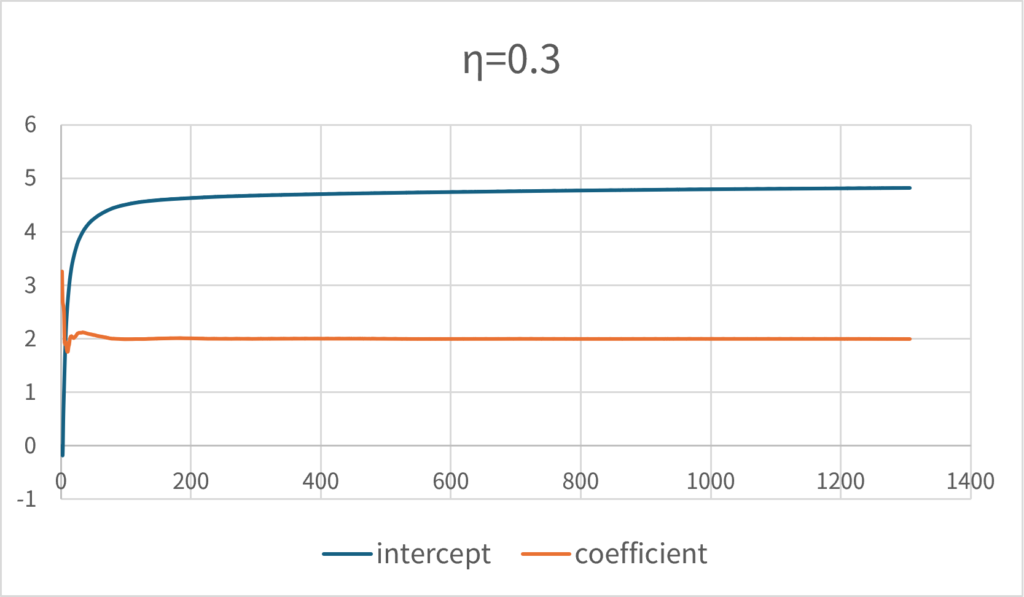
In fact, if you try a one-variable linear regression analysis, you will see that it converges to the correct solution. The following graph shows the progress of parameters when generating simulation paths for \(\small y=2x+5+\epsilon, \epsilon\sim N(0,1)\) and learning the data in order. The learning rate \(\small \eta\) is set to 0.3.

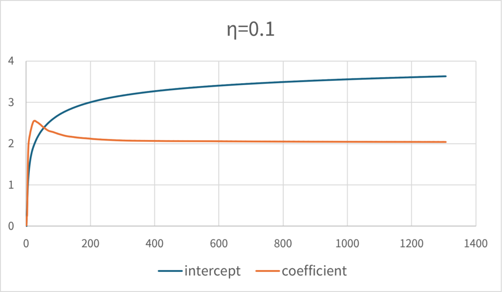
This means that if the learning rate is set low, the convergence rate will be significantly reduced. If \(\small \eta=0.1\), the same number of tries will not converge to the correct solution.

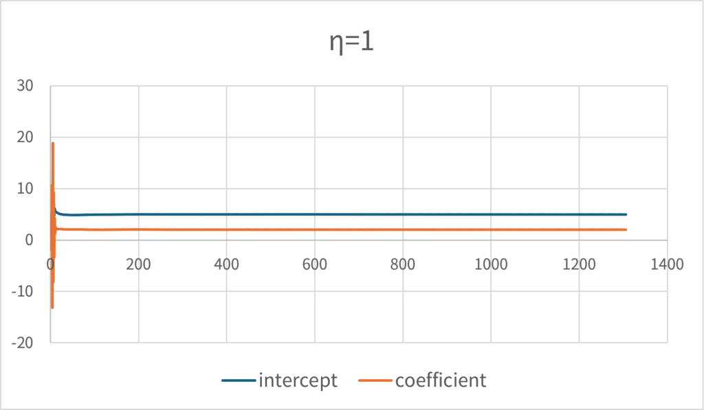
Conversely, it should be noted that if the learning rate is set too high, the solution is likely to diverge. \(\small \eta=1\) eventually converges to a close to the correct solution, but you can see that the parameters fluctuate to a considerable extent in the initial stage.

This approach has poor convergence properties as the number of parameters increases, so it is necessary to repeatedly update the parameters using the same data. The stochastic gradient descent algorithm does this using a random data set. Setting the learning rate higher will improve convergence, but it also increases the risk of the solution diverging, so it is important to set an appropriate value. Repeatedly using the same data to update parameters is likely a process that requires a large amount of computational resources.
Online Machine Learning
Sometimes we want to update the parameters of a regression model using sequentially observed data. Typically, when analyzing data in which the model parameters tend to change over time (non-stationary time series data), the problem is to estimate the model parameters so that they reflect the most recent observed data. In such cases, rather than continuing to use the parameters estimated by performing estimation processing all at once (offline), a method is used in which learning data is input sequentially and the parameters are continually updated online. This type of regression analysis and machine learning technique is called online machine learning.
There seem to be two methods for doing this: the stochastic gradient descent method mentioned in the previous section, and recursive least squares using a Kalman filter. When using stochastic gradient descent, it will be necessary to take measures such as increasing the probability that the most recent observed data is sampled. The method using the Kalman filter is a method in which the variance-covariance matrix of the data is calculated in advance, and the optimal parameter transition is predicted based on the calculated matrix. It should be noted that the recursive least squares method requires the calculation of an inverse matrix during the calculation process, and therefore if there is no method that can efficiently approximate this inverse matrix, the computational cost will be the same as performing a regular regression analysis again.
I don’t think these calculation methods for regression analysis are very well known in general. In reality, unless the model is a regression model with a large number of parameters, the only processing required to estimate the parameters is to solve the normal equations (simultaneous equations) once, so it appears that selecting the appropriate data and recalculating the parameters all at once will make the calculation process faster. The reason why techniques such as stochastic gradient descent for linear regression analysis and recursive least squares are not widely known is probably because they have few practical uses.


Comments