Probability Distribution of Composite Functions
Before getting into the main topic, note that when a random number \(\small x\) follows the probability density function \(\small p_f(x)\), the probability density function of the probability distribution followed by the value mapped by the continuous function \(\small y=g(x)\) can be calculated using
\[ \small p_g(y) = p_f(g^{-1}(y))\frac{dg^{-1}(y)}{dy}. \]
Proofs can usually be found in probability or statistics textbooks. In a previous post, I wrote that the probability distribution followed by \(\small y=g(x)=\sqrt{x}\) follows
\[ \small p_g(x) = p_{x^2}(x^2)\frac{dg^{-1}(x)}{dx} = p_{x^2}(x^2)\frac{dx^2}{dx}=2xp_{x^2}(x^2), \]
and this is the result of extending this to general functions.
1-dimensional Sphere
Let us consider the probability distribution that
\[ \small \begin{align*} &\hat{x} = \frac{x}{\sqrt{x^2+y^2}} \\ &\hat{y} = \frac{y}{\sqrt{x^2+y^2}} \ \end{align*} \]
follow when two standard normal random numbers \(\small x,y\sim N(0,1)\) are given. It may be possible to derive these probability distributions by performing calculations using variable transformations, etc., but this may be surprisingly difficult (incidentally, I was unable to do the calculations). However, since \(\small \hat{x}^2+\hat{y}^2=1\) and \(\small \hat{x},\hat{y}\) are spherically symmetric, it can be inferred that the result will be equivalent to that of calculation:
\[ \small \begin{align*} &\hat{x} = \cos \eta \\ &\hat{y} = \sin \eta, \quad \eta\sim U[0,2\pi]. \end{align*} \]
\(\small U\) represents the uniform distribution. Since the domain of the inverse trigonometric functions is \(\small [-1,1]\), the probability density function of \(\small \hat{x}\) can be obtained as:
\[ \small p(\hat{x}) = \frac{\frac{d\cos^{-1}\hat{x}}{d\hat{x}}}{\int_{-1}^1\frac{d\cos^{-1}\hat{x}}{d\hat{x}}dx} = \frac{1}{\pi \sqrt{1-\hat{x}^2}}. \]
In fact, if you try it using a Monte Carlo simulation, you can confirm that this result is correct. In addition, when we calculate the covariance of \(\small \hat{x},\hat{y}\), it is:
\[ \small E[\hat{x}\hat{y}] =\frac{1}{2\pi}\int_0^{2\pi}\sin\eta\cos\eta d\eta = 0, \]
so we can see that the correlation coefficient of \(\small \hat{x},\hat{y}\) is 0.
2-dimensional Sphere
Similarly, consider the probability distribution that
\[ \small \begin{align*} \hat{x} = \frac{x}{\sqrt{x^2+y^2+z^2}} \\ \hat{y} = \frac{y}{\sqrt{x^2+y^2+z^2}} \\ \hat{z} = \frac{z}{\sqrt{x^2+y^2+z^2}} \end{align*} \]
follows when three standard normal random numbers \(\small x,y,z\sim N(0,1)\) are given. This also has a domain of \(\small [-1,1]\), but because it is spherically symmetric (the probability distribution does not change even if the coordinate axes are swapped), it can be expressed as:
\[ \small \begin{align*} &\hat{x} = \sin \varphi \cos \eta \\ &\hat{y} = \sin \varphi \sin \eta \\ &\hat{z} = \cos \varphi, \qquad \quad \varphi\sim F(\varphi), \quad \eta\sim U[0,2\pi] \end{align*} \]
using polar coordinates. Here, \(\small F(\varphi)\) is a probability distribution whose probability density function and probability distribution function are:
\[ \small \begin{align*} &p_F(\varphi) = \frac{1}{2}\sin \varphi \\ &F(\varphi) = \int p_F(\varphi)d\varphi = \frac{1}{2}(1-\cos \varphi), \quad \varphi \in[0,\pi], \end{align*} \]
respectively. Since it is spherically symmetric, we need to find the probability distribution of \(\small \hat{z}\). It can be calculated as:
\[ \small p(\hat{z}) = \frac{\frac{1}{2}\sin\cos^{-1} \hat{z} \frac{d\cos^{-1} \hat{z}}{d\hat{z}}}{\int_{-1}^1\frac{1}{2}\sin\cos^{-1} \hat{z} \frac{d\cos^{-1} \hat{z}}{d\hat{z}}{d\hat{z}}} = \frac{1}{2} \]
and since the probability density function is a constant, we can see that the probability distribution of \(\small \hat{z}\) is a uniform distribution \(\small U[-1,1]\). Since it is spherically symmetric, \(\small \hat{x},\hat{y}\) also follows a uniform distribution.
3-dimensional Sphere
Similarly, consider the probability distribution that
\[ \small \begin{align*} &\hat{x} = \frac{x}{\sqrt{x^2+y^2+z^2+s^2}} \\ &\hat{y} = \frac{y}{\sqrt{x^2+y^2+z^2+s^2}} \\ &\hat{z} = \frac{z}{\sqrt{x^2+y^2+z^2+s^2}} \\ &\hat{s} = \frac{s}{\sqrt{x^2+y^2+z^2+s^2}} \end{align*} \]
follows when four standard normal random numbers \(\small x,y,z,s \sim N(0,1)\) are given. This also has a domain of \(\small [-1,1]\), but because it is spherically symmetric (the probability distribution does not change even if the coordinate axes are swapped), it can be expressed as:
\[ \small \begin{align*} &\hat{x} = \sin \theta \sin \varphi \cos \eta \\ &\hat{y} = \sin \theta \sin \varphi \sin \eta \\ &\hat{z} = \sin \theta \cos \varphi \\ &\hat{s} = \cos \theta, \qquad \quad \theta\sim G(\theta), \quad\varphi\sim F(\theta), \quad \eta\sim U[0,2\pi] \end{align*} \]
using polar coordinates. Here, \(\small G(\theta)\) is a probability distribution whose probability density function and probability distribution function are:
\[ \small \begin{align*} &p_G(\theta) = \frac{2}{\pi}\sin^2 \theta \\ &G(\theta) = \int p_G(\theta)d\theta = \frac{1}{\pi}(\theta-\sin \theta\cos \theta), \quad \theta \in[0,\pi], \end{align*} \]
respectively. Since it is spherically symmetric, we need to find the probability distribution of \(\small \hat{s}\). It can be calculated as:
\[ \small p(\hat{s}) = \frac{\frac{2}{\pi}\sin^2\cos^{-1}\hat{s} \left(\frac{d\cos^{-1} \hat{s}}{d\hat{s}}\right)}{\int_{-1}^1\frac{2}{\pi}\sin^2\cos^{-1}\hat{s} \left(\frac{d\cos^{-1} \hat{s}}{d\hat{s}}\right){d\hat{s}}} =\frac{2}{\pi}\sqrt{1-\hat{s}^2}. \]
Since it is spherically symmetric, the same probability distribution follows for \(\small \hat{x},\hat{y},\hat{z}\). At this point, it seems possible to generalize to the \(\small n\)-dimensional sphere, so we can infer
\[ \small p_n(\hat{x}) =\frac{(1-\hat{x}^2)^{\frac{n-2}{2}}}{\int_{-1}^1 (1-\hat{x}^2)^{\frac{n-2}{2}} d\hat{x}}. \]
When I tested the program, this result seemed correct.
Conditional Probability Distribution
So far we have dealt with spherically symmetric probability distributions, but what is of interest is the case where the value on one of the coordinate axes is a constant rather than a normal random number. For example, on a 3-sphere, what is the probability distribution of \(\small \hat{x},\hat{y},\hat{z},\hat{s}\) if \(\small s\) is a constant? The probability distribution will be asymmetric only in the \(\small \hat{s}\) direction. Let us calculate the probability distribution in this case.
As usual, let us start with the example of a one-dimensional sphere. Assume that the value is already determined as \(\small y=\bar{y}\). In this case, let us calculate the probability distribution of coordinate
\[ \small \begin{align*} &\hat{x} = \frac{x}{\sqrt{x^2+\bar{y}^2}} \\ &\hat{y} = \frac{\bar{y}}{\sqrt{x^2+\bar{y}^2}}, \quad x\sim N(0,1) \end{align*} \]
on the one-dimensional sphere. If we put \(\small \hat{x} = g(x)\), then its inverse function is:
\[ \small g^{-1}(\hat{x}) =\pm\frac{\hat{x}\bar{y}}{\sqrt{1- \hat{x}^2}}. \]
Hence, we can get
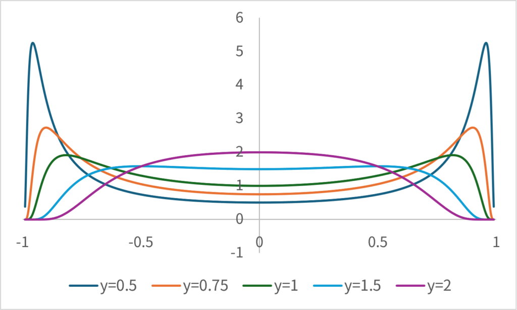
\[ \small p(\hat{x}|y=\bar{y}) \propto \frac{1}{\sqrt{2\pi}}\exp\left(-\frac{\hat{x}^2\bar{y}^2}{2(1-\hat{x}^2)} \right)|\bar{y}|(1- \hat{x}^2)^{-\frac{3}{2}}. \]
When actually calculating, the function becomes as follows:
Similarly, Since we find \(\small p(\hat{y})\), the answer is:
\[ \small g^{-1}(\hat{y}) =\pm\frac{\bar{y}\sqrt{1-\hat{y}^2}}{\hat{y}}, \]
therefore,
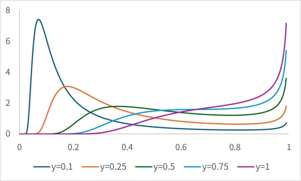
\[ \small p(\hat{y}|y=\bar{y}) \propto \frac{1}{\sqrt{2\pi}}\exp\left(-\frac{(1-\hat{y}^2)\bar{y}^2}{2\hat{y}^2} \right)\frac{|\bar{y}|}{\hat{y}^2\sqrt{1-\hat{y}^2}} \]
can be obtained. However, the domain of definition for \(\small \bar{y}\) and \(\small \hat{y}\) is only the region where the sign is the same. When actually calculating, the function becomes as follows:
Unfortunately, I do not know how to theoretically derive equations for two or more dimensions. However, based on the results of Monte Carlo simulations, I can infer that the following holds true. In the two and three-dimensional cases,
\[ \small \begin{align*} &p(\hat{x}|z=\bar{z}) \propto \frac{1}{\sqrt{2\pi}}\exp\left(-\frac{\hat{x}^2\bar{z}^2}{2(1-\hat{x}^2)} \right)|\bar{z}|(1-\hat{x}^2)^{-3/4} \\ &p(\hat{x}|s=\bar{s}) \propto \frac{1}{\sqrt{2\pi}}\exp\left(-\frac{\hat{x}^2\bar{s}^2}{2(1-\hat{x}^2)} \right)|\bar{s}| \ \end{align*} \]
holds. From this, it seems likely that if we extend it to the \(\small n\)-dimensional sphere, it will be:
\[ \small p_n(\hat{x}_j|x_n=\bar{x}_n, j=1,\cdots,n-1) \propto \frac{1}{\sqrt{2\pi}}\exp\left(-\frac{\hat{x}_j^2\bar{x}_n^2}{2(1-\hat{x}_j^2)} \right)|\bar{x}_n|(1-\hat{x}_j^2)^{(n-3)3/4}. \]
The results of Monte Carlo simulations seem correct for general \(\small n\).
The asymmetric coordinate axis can be inferred to be
\[ \small \begin{align*} &p(\hat{z}|z=\bar{z}) \propto \frac{1}{\sqrt{2\pi}}\exp\left(-\frac{(1-\hat{z}^2)\bar{z}^2}{2\hat{z}^2} \right)\frac{|\bar{z}|}{\hat{z}^3} \\ &p(\hat{s}|s=\bar{s}) \propto \frac{1}{\sqrt{2\pi}}\exp\left(-\frac{(1-\hat{s}^2)\bar{s}^2}{2\hat{s}^2} \right)\frac{|\bar{s}|}{\hat{s}^4}(1-\hat{s}^2)^{\frac{1}{2}} \end{align*} \]
from the results of a Monte Carlo simulation. When expanded to a \(\small n\)-dimensional sphere,
\[ \small p_n(\hat{x}_n|x_n=\bar{x}_n) \propto \frac{1}{\sqrt{2\pi}}\exp\left(-\frac{(1-\hat{x}_n^2)\bar{x}_n^2}{2\hat{x}_n^2} \right)|\bar{x}_n|\hat{x}_n^{-(n+1)}(1-\hat{x}_n^2)^{(n-2)/2} \]
can be calculated. I would like to come up with an elegant proof someday, but I can’t think of one right now…


Comments