Introduction
There are two types of Texas Hold’em: ring games, in which chips acquired from other players are used to win, and tournaments, in which players compete to see who can survive the longest, with prize money awarded according to their ranking. In ring games, you play to maximize the expected value of your chips (although I have some doubts about this approach), but in tournaments you need to maximize the expected value of the prize money you receive as a result of competing for ranking. To calculate this, we need to calculate the probability of ranking given the current stack distribution of players. This article introduces a model to estimate it.
ICM (Independent Chip Model)
Assume there are \(\small n\) players with stacks \(\small s_1,\cdots,s_n\) each. In this case, we assume that player \(\small i\)’s probability of winning is proportional to his or her current stack. If we express that the first-ranked player is \(\small i\) as \(\small r_1 = 1\), then the probability that player \(\small i\) wins can be expressed as:
\[ \small p_i^{(1)} = \text{Pr}[r_1=i] = \frac{s_i}{\sum_{z=1}^n s_z}. \]
Furthermore, suppose that the probability that the second place player is \(\small j\) when the first place player is \(\small i\) is proportional to the stack excluding \(\small i\)’s stack, and assume that this is given by
\[ \small p_{ij}^{(2)} = \text{Pr}[r_2 = j \:|\:r_1=i] = \frac{s_j}{\sum_{z=1,z\neq i}^n s_z}. \]
In this case, it is easy to see that regardless of who the first place player is, the probability that the second place player is \(\small j\) can be calculated using
\[ \small p_j^{(2)} = \sum_{i=1, i\neq j}^n p_{ij}^{(2)}. \]
The probability of coming in third place and beyond can be calculated in the same way. Suppose the probability that the third place player is \(\small k\) when the first place player is \(\small i\) and the second place player is \(\small j\) is given by
\[ \small p_{ijk}^{(3)} = \text{Pr}[r_3 = k \:|\:r_1=i,r_2=j] = \frac{s_j}{\sum_{z=1,z\neq i,j}^n s_z}. \]
In this case, regardless of who the first and second place players are, the probability that the third place player is \(\small k\) can be calculated as:
\[ \small p_k^{(3)} = \sum_{i=1, i\neq k}^n \sum_{j=1, j\neq i,k}^n p_{ijk}^{(3)}. \]
By repeating this process, we can determine all the probabilities of what place a player with stack \(\small s\) will come in.
This method of calculating the probability of a player’s ranking is called the Independent Chip Model (ICM). The above calculations implicitly assume that the probability that two players have a ranking of \(\small i<j\) is not affected by the presence of another player \(\small k\). In decision theory, this assumption is called Independence from Irrelevant Alternatives (IIA). This assumption is often used to estimate the probability of winning in gambling on the rankings of horse races and boat races. In economics, this condition is often assumed when determining the ranking of options through voting, such as in social choice theory (although it is often criticized for this).
It is important to note that, as can be seen from the structure of the formula above, the computational complexity of this calculation grows exponentially as the number of players \(\small n\) increases. Therefore, exact calculations are possible only when \(\small n\) is small, and when \(\small n\) is large, the only way to calculate the approximate value is to use Monte Carlo simulation. The method of calculating with Monte Carlo simulation will be described later.
Tournament Prize Model
ICM is used as the objective function in tournaments where the prize money is determined by the ranking of players, not the amount of chips earned, so it is important to consider how much prize money the tournament allocates to each ranking. This generally tends to be roughly determined according to a power function. This is what I mentioned in my previous post on the Pareto principle.
I mentioned that workers’ incomes are determined by a function close to a power function, and tournament prize money is determined in a similar way. Perhaps determining compensation in this way serves to motivate many people, as businesspeople and poker players are similar in the sense that they are both incentivized and exploited by bookmakers.
Let’s use a simple example to illustrate the calculation method. Assume that there are 100 participants in a tournament, with each participant paying a $100 entry fee. The total amount bet is $10,000, and the prize money to be distributed is $9,000, minus 10%, or $1,000, as the casino’s commission. We assume that the top 10 players will receive the prize money, and we will set the prize money for each ranking so that the total amount is $9,000.
Let’s define the prize money that the winner can receive as \(\small W_1\), and the prize money for second place and below as:
\[ \small W_m = \frac{W_1}{\beta^{m-1}}, \quad \beta>1. \]
In this case, we just need to determine the values of \(\small W_1\) and \(\small \beta\) so that the total prize amount is:
\[ \small W = \sum_{m=1}^{10} W_m = 9000. \]
In this case, it would be sufficient to set \(\small \beta\) so that the prize money received by the 10th place winners exceeds the entry fee. The upper limit of \(\small \beta\) is around 1.45, but let’s use \(\small \beta=1.35\) here to calculate the prize money for each ranking. Specifically, it can be calculated as follows:
| Ranking | 1/β^(m-1) | Prize Money |
|---|---|---|
| 1 | 1 | 2455 |
| 2 | 0.74074 | 1819 |
| 3 | 0.54870 | 1347 |
| 4 | 0.40644 | 998 |
| 5 | 0.30107 | 739 |
| 6 | 0.22301 | 548 |
| 7 | 0.16520 | 406 |
| 8 | 0.12237 | 300 |
| 9 | 0.09064 | 223 |
| 10 | 0.06714 | 165 |
From the probability that player \(\small i\) will rank \(\small m\) calculated from ICM and the prize amount \(\small W_m\) that player \(\small i\) can receive when ranked \(\small m\), the expected prize amount \(\small R_i\) that player \(\small i\) can receive can be calculated as:
\[ \small R_i(s) = \sum_{m=1}^{10} p_i^{(m)}(s) W_m. \]
\(\small s\) is the vector of stacks of all players. In a tournament, instead of maximizing the expected value of the stacks, you need to devise a betting strategy to maximize this \(\small R_i(s)\).
Estimation using Monte Carlo Simulation
The exact calculation of ICM requires an exponential increase in the amount of computation required with respect to the number of participants \(\small n\), but it can be easily calculated using Monte Carlo simulation (although simulation errors will occur). Simply put, you can randomly select the first place player from the probability distribution calculated from the stack, then randomly select the second place player from the probability distribution excluding the first place player, and repeat this process to easily estimate the probability distribution of what place each player will get. I’ve posted the source code implemented in Python. It seems that the source code was written by ChatGPT…
import random

def calc_icm(stack, n_simulation):
    n = len(stack)
    r = [[0 for _ in range(n)] for _ in range(n)]

    # Normalized Probability Vector
    total = sum(stack)
    p = [s / total for s in stack]

    for _ in range(n_simulation):
        ranking = []
        q = [0] * n

        for _ in range(n):
            # Calculate the total probability of remaining players
            remaining_indices = [k for k in range(n) if k not in ranking]
            remaining_total = sum(p[k] for k in remaining_indices)

            # Update q (current probability of being selected)
            for k in range(n):
                q[k] = p[k] / remaining_total if k in remaining_indices else 0.0

            # Randomly select one player
            v = random.random()
            acc = 0
            for k in range(n):
                acc += q[k]
                if v <= acc and q[k] > 0:
                    ranking.append(k)
                    break

        # Add the ranking result to r
        for position, player in enumerate(ranking):
            r[player][position] += 1

    # Averaging
    for i in range(n):
        for j in range(n):
            r[i][j] /= n_simulation

    return r

if __name__ == "__main__":
    # Example: There are 4 players, each with the following stack amounts:
    stack = [1000, 1500, 2000, 500]

    # Number of simulations (the higher the number, the higher the accuracy)
    n_simulation = 10000

    # Perform an ICM calculation
    icm_result = calc_icm(stack, n_simulation)

    # Show the results
    print("ICM Probability Distribution (rows: players, columns: ranks)")
    for i, row in enumerate(icm_result):
        print(f"Player{i+1}: " + " ".join(f"{prob:.4f}" for prob in row))
To give a concrete example, let’s say there are 10 players remaining, each with a stack of
\[ \small s = \{s_1,\cdots,s_{10}\} = \{18,16,14,12,11,9,8,6,4,2\}. \]
Let’s calculate each player’s expected prize amount \(\small R_i(s)\) in this case. If we arrange these in stack order, we can find the shape of the expected prize function \(\small R(s)\) for stacks. The ICM-estimated probability of each player’s placement is as follows:
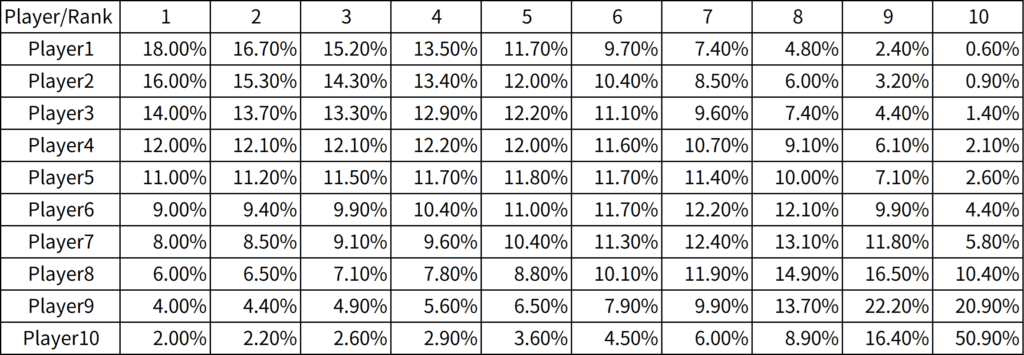
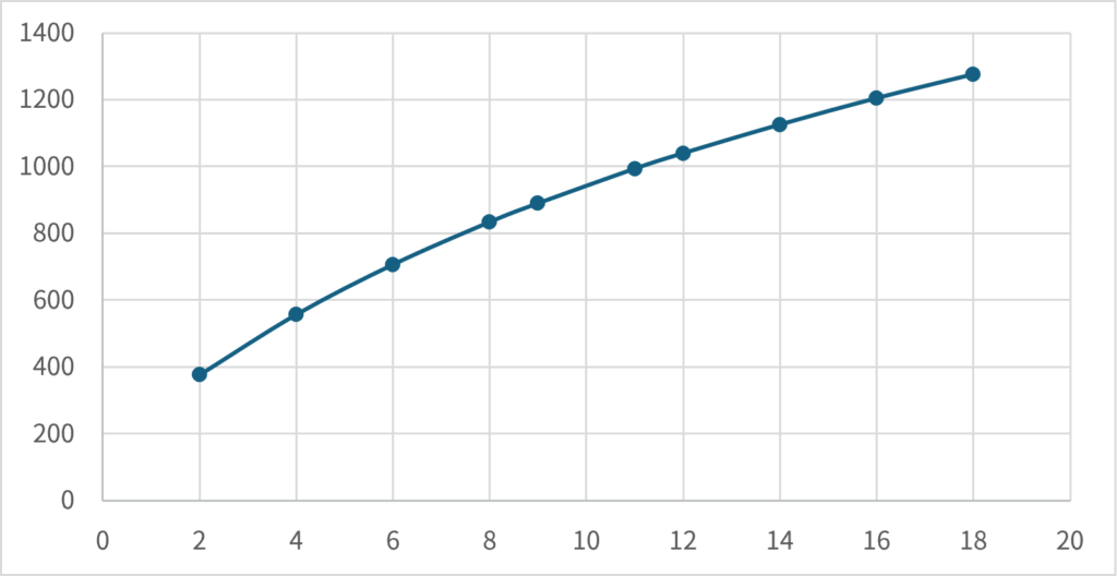
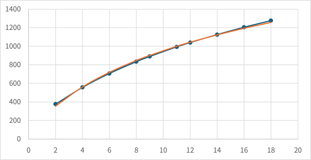
Assume that the prize amounts for 1st through 10th place are given in the table in the previous section. We calculate each player’s expected prize amount \(\small R_i(s)\), and plot it against their stack \(\small s\) as follows:
Power Utility Function (CRRA Type Utility Function)
Looking at the graph from the previous section, you can see that the expected prize is an upward convex function of the stack \(\small s\). In other words, if we consider the expected winnings as a utility function with respect to the stack \(\small s\), we can infer that it is optimal to be risk-averse with respect to the stack \(\small s\). In addition, the shape of the graph shows that it is similar to the shape of the function when \(\small \gamma < 1\) is set for the CRRA utility function:
\[ \small U(s) = \frac{s^{1-\gamma}-1}{1-\gamma}. \]
A CRRA-type utility function where \(\small \gamma < 1\) is called a power utility function. In this case, even if \(\small s=0\), \(\small U(s)\) can be calculated as a finite value, so it can be used as a utility function expressing risk aversion even in games such as Texas Hold’em where the stack can become zero.
In fact, if you approximate the graph in the previous section using a function with \(\small \gamma = 0.25\), you can see that it roughly matches (we estimated it using \(\small 1/1.35 \approx 0.74 \approx 1-\gamma\), but \(\small \gamma\) needs to be set smaller as the number of players increases). The orange line is a graph of the (linearly transformed) values obtained by setting the power utility function as \(\small U(s) = s^{1-0.25}\) and determining \(\small a,b\) so that the squared error is minimized in \(\small R(s) = a + b U(s)\).
Many textbook Texas Hold’em strategies are calculated to maximize the expected value of your stack (\(\small \gamma=0\)), making them too risky to use in tournament situations. This means that you need to adjust your pre-flop hand range and betting strategy according to your risk aversion. Of course, when there are many players left and most of them are not going to win money, you don’t need to make such calculations and you can just play to maximize the expected value of your stack. On the other hand, if you see yourself coming in higher, you’ll need to choose your cards in a more risk-averse way (for example, not going all-in preflop with a mediocre hand even if you’re short stacked) and adjust your bet amount in order to survive as many games as possible and aim for a higher ranking.


Comments