
Introduction
Along with free particles, a typical example of calculation using the Schrödinger equation is the harmonic oscillator, which is the subject of this article. The mathematical calculations are extremely difficult, and in almost all textbooks there is no explanation as to why these calculations are justified. This seems to be a typical example of a “shut up and calculate” problem. However, It is also famous as the calculation that justifies the fact that the energy of a photon can only take on discrete values such as
\[ E_n = \left(n+\frac{1}{2} \right)\hbar \omega, \]
and unless we truly understand this, it is likely that quantum mechanics will remain poorly understood. Furthermore, most textbooks are satisfied with deriving the above energy, and end up not showing what kind of probability distribution the Schrödinger equation for the harmonic oscillator expresses (or rather, they show an incorrect probability distribution). In this article, I will go as far as calculating the final probability distribution and present my own interpretation of the solution, which is largely hypothetical, based on my own arbitrary and biased views.
Formulation
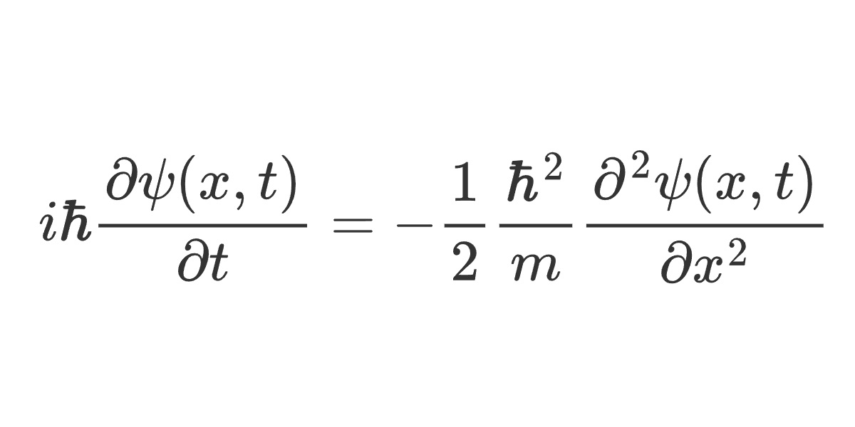
Let us find a solution to the Schrödinger equation:
\[ i\hbar\frac{\partial\psi(x,t)}{\partial t} = -\frac{\hbar^2}{2m}\frac{\partial^2\psi(x,t)}{\partial x^2}+\frac{m}{2}\omega^2x^2\psi(x,t) \]
derived by applying the correspondence principle:
\[ E \rightarrow i\hbar\frac{\partial}{\partial t}, \quad p \rightarrow i\hbar\frac{\partial}{\partial x} \]
in quantum mechanics to the harmonic oscillator:
\[ E = \frac{p^2}{2m} + \frac{m}{2}\omega^2x^2 \]
in classical mechanics. Let assume a function that is separable in \(\small x,t\) similar to the wave function in the free state:
\[ \psi(x,t) = \exp\left(i\frac{p}{\hbar}x\right)\exp\left(-i\frac{E}{\hbar} t \right). \]
In other words, let assume
\[ \psi(x,t) = \Psi(x)\exp\left(-i\frac{E}{\hbar} t \right). \]
This allows the Schrödinger equation for the harmonic oscillator to be replaced by
\[ E\Psi(x) = -\frac{\hbar^2}{2m}\frac{d^2\Psi(x)}{dx^2}+\frac{m}{2}\omega^2x^2\Psi(x). \]
By rearranging the equation,
\[ \frac{d^2\Psi(x)}{dx^2}+\left(\frac{2m}{\hbar^2}E-\frac{m^2\omega^2}{\hbar^2}x^2\right)\Psi(x) = 0 \]
can be obtained.
Hermite Polynomials
In order to find the solution to the differential equation in the previous section, we will briefly introduce the definition of Hermite polynomials. Polynomials that satisfy the formula:
\[ H_n(\xi) = (-1)^ne^{\xi^2} \frac{d^n}{d\xi^n}e^{-\xi^2} \]
are called Hermite polynomials. The specific function type is expressed using a special function called a confluent hypergeometric function, but this is not used in this article so you do not need to worry about it. Let us just recognize that it is a polynomial calculated from the formula. An interesting property of Hermite polynomials is that when \(\small \exp(-(\xi-a)^2)\), which is a normal distribution function, is expanded into a Taylor series,
\[ \begin{align*} \exp\left(-(\xi-a)^2\right) &=\exp\left(-\xi^2 \right)\exp\left(2\xi a-a^2 \right) \\ &=\exp\left(-\xi^2 \right) \sum_{n=0}^{\infty} \frac{1}{n!}H_n(\xi)a^n \end{align*} \]
holds. Hermite polynomials are known to satisfy the following differential equation:
\[ \frac{d^2H_n(\xi)}{d\xi^2}-2\xi\frac{dH_n(\xi)}{d\xi}+2nH_n(\xi)=0,\quad n=0,1,\cdots. \]
Let us transform the differential equations from the previous section to correspond to this form.
Let us define the notation:
\[ k^2 = \frac{2mE}{\hbar^2},\quad \lambda = \frac{m\omega}{\hbar},\quad\xi = \sqrt{\lambda}x. \]
This allows the problem equation to be transformed with
\[ \begin{align*} &\lambda\frac{d^2\Psi(\xi)}{d\xi^2}+\left(k^2-\lambda \xi^2\right)\Psi(\xi) = 0 \\ \Rightarrow & \frac{d^2\Psi(\xi)}{d\xi^2}+\left(\frac{k^2}{\lambda}-\xi^2\right)\Psi(\xi) = 0. \end{align*} \]
Assuming
\[ \Psi(\xi) = \exp\left(-\frac{\xi^2}{2} \right) \Phi(\xi) \]
is the solution form of \(\small \Psi(\xi)\), let us find the differential equation for \(\small \Phi(\xi)\). Steady calculations reveal that
\[ \frac{d^2\Psi(\xi)}{d\xi^2} = \exp\left(-\frac{\xi^2}{2} \right) \left[(\xi^2-1) \Phi(\xi)-2\xi\frac{d\Phi(\xi)}{d\xi}+\frac{d^2\Phi(\xi)}{d\xi^2}\right] \]
holds true, and by substituting it into the original equation we get
\[ \frac{d^2\Phi(\xi)}{d\xi^2}-2\xi\frac{d\Phi(\xi)}{d\xi}+\left(\frac{k^2}{\lambda}- 1\right)\Phi(x) = 0. \]
Considering the correspondence between Hermite polynomials and differential equations, if
\[ 2n = \frac{k^2}{\lambda}-1 \]
holds, then the solution to \(\small \Phi(\xi)\) can be determined as a linear combination of
\[ \Phi_n(\xi) = H_n(\xi), \quad n=0,1,\cdots. \]
Substituting the defining formula gives us
\[ 2n = \frac{2E_n}{\hbar\omega}-1, \]
so it would be sufficient if
\[ E_n = \left(n+\frac{1}{2}\right)\hbar\omega \]
were true.
Therefore, the basis function of the wave function can be defined as:
\[ \psi_n(\xi(x),t) = \exp\left(-\frac{\xi^2}{2}\right)H_n(\xi)\exp\left(-i\frac{E_n}{\hbar} t \right). \]
Finally, a general solution can be obtained as:
\[ \psi(x,t) = \sum_{n=0}^\infty A_n \psi_n(\xi(x),t), \]
which is expressed as a linear combination of these basis functions.
Gaussian Wave Packet Model
Most textbooks present the probability distribution represented by the Schrödinger equation for a harmonic oscillator as a probability distribution derived from a single Hermite polynomial, for example, the following figure:
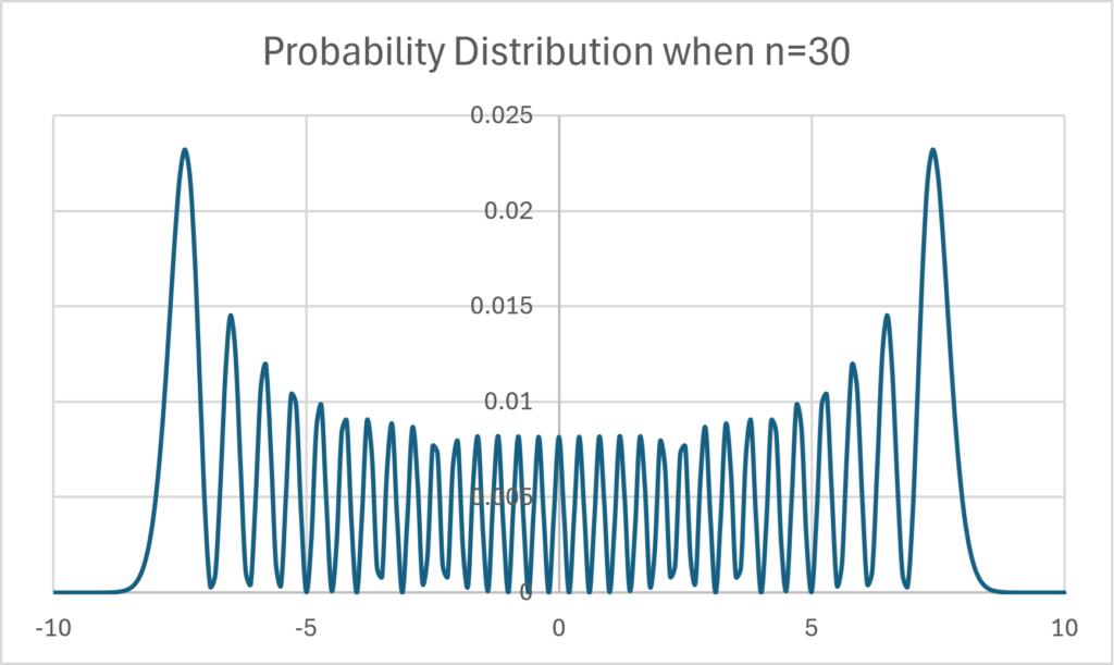
Looking at this, you might think that the probability distribution of the coordinates of a quantum (photon) is indeed discrete, but this is incorrect. Hermite polynomials are merely basis functions for expressing probability distributions, and do not by themselves represent the probability distribution of photon detection. As written at the end of the previous section, in order to calculate this we must calculate
\[ \psi(x,t) = \sum_{n=0}^\infty A_n \psi_n(\xi(x),t). \]
Similar to the Schrödinger equation in the free state, we assume that the uncertainty in the photon’s coordinates at the initial instant is represented by a normal distribution. Since the Hermite polynomials are related to the Taylor expansion of the normal distribution by
\[ \exp\left(-(\xi-a)^2\right) =\exp\left(-\xi^2 \right) \sum_{n=0}^{\infty} \frac{1}{n!}H_n(\xi)a^n, \]
we consider
\[ A_n \propto \frac{1}{n!}\left(\frac{a}{2} \right)^n, \quad n=0,1,\cdots \]
to be the value of the probability amplitude \(\small A_k\). Note that if we set \(\small 0!=1\), then we get \(\small A_0 = 1\). \(\small a\) is an arbitrary constant. In this case, the wave function at the initial point is:
\[ \begin{align*} \psi(x, 0) &= \sum_{n=0}^\infty A_n \psi_n(\xi(x),0) = \sum_{n=0}^\infty \frac{1}{n!}\left(\frac{a}{2} \right)^n\exp\left(-\frac{\xi^2}{2}\right)H_n(\xi) \\ & = \exp\left(\frac{\xi^2}{2}\right)\sum_{n=0}^\infty \frac{1}{n!}\exp\left(-\xi^2\right)H_n(\xi)\left(\frac{a}{2} \right)^n. \end{align*} \]
The series part can be replaced by
\[ \exp\left(-\left(\xi-\frac{a}{2} \right)^2 \right)=\sum_{n=0}^\infty \frac{1}{n!}\exp\left(-\xi^2\right)H_n(\xi)\left(\frac{a}{2} \right)^n. \]
Therefore,
\[ \begin{align*} \psi(x, 0) &= \exp\left(\frac{\xi^2}{2}\right) \exp\left(-\left(\xi-\frac{a}{2} \right)^2 \right) \\ &=\exp\left(\frac{a^2}{4}\right)\exp\left(-\frac{\left(\xi-a\right)^2}{2} \right) \end{align*} \]
can be obtained. If we change \(\small \xi\) back to \(\small x\), we get
\[ \psi(x, 0) = \exp\left(\frac{a^2}{4}\right)\exp\left(-\frac{\lambda\left(x-\frac{a}{\sqrt{\lambda}}\right)^2}{2} \right). \]
Since it is a normal distribution, if we define the constant coefficient as:
\[ A_n = \left(\frac{\lambda}{\pi}\right)^{{1/4}}e^{-a^2/4}\frac{1}{n!}\left(\frac{a}{2} \right)^n, \quad n=0,1,\cdots, \]
the sum of the probability distribution of the coordinates will be 1 and we obtain
\[ \begin{align*} &\psi(x, 0) = \left(\frac{\lambda}{\pi}\right)^{{1/4}}\exp\left(-\frac{\lambda\left(x-\frac{a}{\sqrt{\lambda}}\right)^2}{2} \right) \\ &P(x, 0) = |\psi(x, 0)|^2 = \sqrt{\frac{\lambda}{\pi}}\exp\left(-\lambda\left(x-\frac{a}{\sqrt{\lambda}}\right)^2 \right). \end{align*} \]
Let define the normal distribution function as \(\small N(\mu,\sigma^2)\), it can be represented as:
\[ x \sim N \left(\frac{a}{\sqrt{\lambda}}, \frac{1}{2\lambda} \right). \]
If we were to express it in a volatility-like way, it would be \(\small 1/\lambda = \sigma^2\).
In the same way, let us calculate function
\[ \psi(x,t) = \sum_{n=0}^\infty A_n \psi_n(\xi(x),t) \]
including its time evolution. If we calculate it well, we get
\[ \begin{align*} \psi(x, t) &= \left(\frac{\lambda}{\pi}\right)^{{1/4}}e^{-a^2/4}\sum_{n=0}^\infty \frac{1}{n!}\left(\frac{a}{2} \right)^n\exp\left(-\frac{\xi^2}{2}\right)H_n(\xi)\exp\left(-i\frac{E_n}{\hbar} t \right) \\ & = \left(\frac{\lambda}{\pi}\right)^{{1/4}}e^{-a^2/4}\exp\left(\frac{\xi^2-i\omega t}{2}\right)\sum_{n=0}^\infty \frac{1}{n!}\exp\left(-\xi^2\right)H_n(\xi)\left(\frac{a}{2}e^{-i\omega t} \right)^n. \end{align*} \]
The series part is replaced as:
\[ \exp\left(-\left(\xi-\frac{a}{2}e^{-i\omega t} \right)^2 \right)=\sum_{n=0}^\infty \frac{1}{n!}\exp\left(-\xi^2\right)H_n(\xi)\left(\frac{a}{2}e^{-i\omega t} \right)^n \]
from Taylor expansion. Therefore,
\[ \psi(x,t) = \left(\frac{\lambda}{\pi}\right)^{{1/4}}e^{-a^2/4}\exp\left(\frac{a^2}{4}e^{-2i\omega t}-\frac{i\omega t}{2} \right)\exp\left(-\frac{\left(\xi-ae^{-i\omega t}\right)^2}{2} \right) \]
can be obtained. If we change \(\small \xi\) back to \(\small x \), we get
\[ \psi(x, t) = \left(\frac{\lambda}{\pi}\right)^{{1/4}}e^{-a^2/4}\exp\left(\frac{a^2}{4}e^{-2i\omega t}-\frac{i\omega t}{2} \right)\exp\left(-\frac{\lambda\left(x-\frac{a}{\sqrt{\lambda}}e^{-i\omega t}\right)^2}{2} \right). \]
If we multiply it by the complex conjugate and calculate the probability distribution of the coordinates,
\[ P(x, t) = |\psi(x, t)|^2 = \sqrt{\frac{\lambda}{\pi}}\exp\left(-\lambda\left(x-\frac{a}{\sqrt{\lambda}}\cos\omega t\right)^2 \right) \]
can be obtained. The calculation is a little complicated, but it can be derived using relational equation:
\[ (\cos \omega t)^2= \frac{1}{4}(e^{-2i\omega t} + e^{2i\omega t}+2). \]
By using the normal distribution function,
\[ x(t) \sim N\left(\frac{a}{\sqrt{\lambda}}\cos\omega t, \frac{1}{2\lambda} \right) \]
can be obtained. This is the probability distribution of coordinates represented by the Schrödinger equation for the harmonic oscillator. If the time is fixed, the variance is a constant normal distribution, and if we consider it as a stochastic process, the drift can be considered to be an equation that represents a white noise process of a cosine function.
Finally, let us confirm that the above solution satisfies the Schrödinger equation for the harmonic oscillator. Since
\[ \begin{align*} &\frac{\partial^2 \psi(x, t)}{\partial x^2} = \left[\lambda^2\left(x-\frac{a}{\sqrt{\lambda}}e^{-i\omega t}\right)^2-\lambda \right]\psi(x, t) \\ &\frac{\partial \psi(x, t)}{\partial t} = \left[-\frac{i\omega}{2}\left( a^2e^{-2i\omega t}+1\right)+i\omega\lambda\left(x-\frac{a}{\sqrt{\lambda}}e^{-i\omega t}\right)\frac{a}{\sqrt{\lambda}}e^{-i\omega t}\right]\psi(x, t), \end{align*} \]
we can obtain
\[ \begin{align*} &-\frac{\hbar^2}{2m}\frac{\partial^2 \psi(x, t)}{\partial x^2} = \frac{\hbar\omega}{2} \left[-\lambda\left(x-\frac{a}{\sqrt{\lambda}}e^{-i\omega t}\right)^2+1\right]\psi(x, t) \\ &i\hbar\frac{\partial \psi(x, t)}{\partial t} = \frac{\hbar\omega}{2}\left[\left( a^2e^{-2i\omega t}+1\right)-2\lambda\left(x-\frac{a}{\sqrt{\lambda}}e^{-i\omega t}\right)\frac{a}{\sqrt{\lambda}}e^{-i\omega t}\right]\psi(x, t). \end{align*} \]
If we calculate it honestly,
\[ i\hbar\frac{\partial \psi(x, t)}{\partial t}+\frac{\hbar^2}{2m}\frac{\partial^2 \psi(x, t)}{\partial x^2} =\frac{\hbar\omega}{2}\lambda x^2 \]
can be obtained. If we change \(\small \lambda\) back to its original notation, we can confirm that it indeed satisfies the Schrödinger equation for the harmonic oscillator.
Interpretation of the Harmonic Oscillator Solution
Calculations that use harmonic oscillators to describe the equation of motion (Hamiltonian) of the electromagnetic field (photon) are well explained in quantum mechanics, and the phenomenon that the energy of a photon only takes on discrete values is also justified by harmonic oscillator calculations. However, it is said that it is not clear what the significance of this calculation is, or what the background is for it being possible to calculate the physical quantities of an electromagnetic field using this type of calculation, and it is basically incomprehensible to me as well. There are some points that may raise questions, such as the fact that electromagnetic fields (photons) probably have no mass in the first place, and whether it is appropriate to treat them using classical mechanics equations when they move at the speed of light.
Even in the explanation in this digest-like article, although the calculations are extremely time-consuming, the solution that is obtained is a result that can be described by
\[ x(t) = \frac{a}{\sqrt{\lambda}} \cos\omega t + \epsilon(t), \quad \epsilon(t)\sim N\left(0,\frac{1}{2\lambda}\right) \]
if written as a stochastic process. If written in stochastic process theory, the explanation could be completed in one line, as the drift is a white noise process with a cosine function. This may be the intuitive meaning of what a harmonic oscillator represents, as it is how it represents the motion of the electromagnetic field (photons). Below, I will conclude by presenting my hypothesis.
If we accept the validity of the principle of the constancy of the speed of light in the theory of relativity, it does not seem appropriate to consider the above motion as the equation of motion of a photon. Since the speed is constant, if time is one-dimensional, the photon should not be able to move in any direction other than in a straight line, and so it would have to be
\[ x(t) = ct + \epsilon(t), \quad \epsilon(t)\sim N\left(0,\frac{\sigma^2}{2}\right), \]
as derived from the “Schrödinger equation in the free state.” However, if we further add the assumption of the principle of relativity, the assumption that time is one-dimensional is actually incorrect, and it turns out that there must be as many different times as there are coordinates (or particles) being described. The space-time that combines the principle of relativity and the principle of the constancy of the speed of light is a coordinate system called a conical coordinate system (light cone coordinate system):
\[ x^2 + c^2T_{xt}^2=c^2t^2. \]
What we perceive as time is not \(\small t\), but \(\small T_{xt}\), which is expressed as a function of the coordinate \(\small x\). Geometrically speaking, the concept of time is a two-dimensional curved surface (hypersurface). It was Tomonaga Shin-ichiro who first came up with this idea, and it is known as the super-many time theory. The concept of space in this coordinate system is one in which time is fixed as a constant, so if we assume \(\small t=1/c\), we get
\[ x^2 + s^2=1, \]
and the space assumed by the theory of relativity is a sphere \(\small S^1\) (in reality it is a three-dimensional sphere \(\small S^3\)). Since the coordinates on the sphere can be expressed as:
\[ x(t) = \cos \omega t \\ s(t) = \sin \omega t. \]
using trigonometric functions, the original conic coordinate system can be expressed as:
\[ \begin{align*} &x^2 + c^2 T_{xt}^2 = c^2t^2\left(\cos^2\omega t + \sin^2\omega t\right) = c^2t^2 \\ \Rightarrow & x(t) = ct \cos \omega t. \end{align*} \]
Thinking in this way, we might surmise that the solutions derived from the Schrödinger equation for the harmonic oscillator represent coordinates in a conical coordinate system rather than in Euclidean space. In other words, if we think of angular frequency as the inverse of time and set it as \(\small \omega \propto 1/t \), we may be able to define it as:
\[ \frac{a}{\sqrt{\lambda}} = ct \propto \frac{c}{\omega}. \]
Eventually, the detection coordinate (the coordinate in which it interacts with other quanta) of a photon (electromagnetic field) is represented as
\[ x(t) = ct \cos\omega t + \epsilon(t), \quad \epsilon(t)\sim N\left(0,\frac{\sigma^2}{2}\right), \]
and we can hypothesize that this is what the Schrödinger equation for the harmonic oscillator represents. The author’s hypothesis is that the motion of photons derived from this is a white noise process in a conical coordinate system, and that the description of the Schrödinger equation for the harmonic oscillator happens to coincide with it, allowing it to be treated as the equation of motion for the electromagnetic field. If we think about it in this way, the Schrödinger equation for the harmonic oscillator does not actually represent a harmonic oscillator, but rather rotational motion on a sphere, where the potential is also
\[ V(x) = \frac{m}{2}\omega^2x^2. \]
The problem is that the name is misleading. Well, that’s not my concern…
Furthermore, if we consider the concept of time as a two-dimensional curved surface as described above, doubts arise as to whether it is actually energy that takes on discrete values. In physics, energy is defined as an invariant with respect to time evolution, so it would be unnatural to imagine it as being able to take on probabilistically random values. The original energy of a photon is:
\[ E = \frac{\hbar\omega}{2}, \]
and the value in the form \(\small 2n+1\) may be a different concept. Furthermore, it is thought that the concept we commonly recognize as time is not \(\small t\) but \(\small T_{xt}\). In other words, I speculate that the original form of the wave function is:
\[\exp\left(-i\frac{E_n}{\hbar}T_{xt} \right) = \exp\left(-i\frac{E}{\hbar}\int_0^t\frac{\partial T_{xu}}{\partial u}du \right) \]
and that its derivative with respect to local time \(\small \partial T_{xt}/\partial t \) takes the value given by
\[ \frac{\partial T_{xt}}{\partial t} \approx 1,3,5,7,\cdots. \]
The author’s hypothesis is that because this is recognized as
\[ E_n = E \frac{\partial T_{xt}}{\partial t} \]
in physics experiments, it has become a poorly understood theory.
Reference
[1] Tomonaga, Shin-ichiro (1962). Quantum Mechanics Volume 1:Old Quantum Theory. North-Holland.
[2] Tomonaga, Shin-ichiro (1966). Quantum Mechanics Volume 2:New Quantum Theory. John Wiley & Sons (Interscience Publishing).
[3] Hirano, Kaname (2022), Quantum Mechanics with Multi-Time Theory, Amazon Kindle Store.
[4] Hirano, Kaname (2024), Complex Functions and Schrödinger Equation, Amazon Kindle Store.

Comments