Euler Method
Given an ordinary differential equation:
\[ \small \frac{dx}{dt} = f(x,t),\quad x(0) = x_0 \]
with initial conditions, we consider how to numerically solve this equation. The simplest method would be to discretize the time and perform the calculation. If we define \(\small t_k = k\Delta t, \Delta t = 1/n,x_k=x(t_k)\) and approximate it by difference with
\[ \small \frac{x_{k+1}-x_k}{\Delta t} = f(x_k, t_k), \]
we can find the solution by successively calculating with
\[ \small x_{k+1} = x_k+f(x_k,t_k)\Delta t. \]
This is a numerical method for solving ordinary differential equations known as the Euler method.
The Euler method can also be applied to simultaneous differential equations. In the case of
\[ \small \begin{align*} \frac{dx}{dt} = f(x,y,t),\quad x(0) = x_0 \\
\frac{dy}{dt} = g(x,y,t),\quad y(0) = y_0, \end{align*} \]
we can solve it as:
\[ \small \begin{align*} x_{k+1} = x_k+f(x_k,y_k,t_k)\Delta t \\
y_{k+1} = y_k+g(x_k,y_k,t_k)\Delta t. \end{align*} \]
It can be easily extended to the case of second-order differential equations. If the second-order differential equation is expressed as:
\[ \small \frac{d^2x}{dt^2} = f(x,t)\frac{dx}{dt}+ g(x,t),\quad x(0) = x_0,\;\frac{dx}{dt}(0) = v_0, \]
it can be transformed into
\[ \small \begin{align*} &\frac{dv(x,t)}{dt} = f(x, t)v(x,t)+g(x, t) \\ &\frac{dx(t)}{dt} = v(x,t). \end{align*} \]
Therefore, the solution can be found by performing sequential calculations on
\[ \small \begin{align*} &v_{k+1} = v_k+(f(x_k,t_k)v_k+g(x_k,t_k))\Delta t \\ &x_{k+1} = x_k + v_{k} \Delta t. \end{align*} \]
For example, the simultaneous differential equations:
\[ \small \begin{align*} &\frac{d^2x}{dt^2} = -\frac{GM}{r^3}x \\ &\frac{d^2y}{dt^2} = -\frac{GM}{r^3}y \\ &\frac{d^2z}{dt^2} = -\frac{GM}{r^3}z \end{align*} \]
which are used to calculate gravity can be calculated as:
\[ \small \begin{align*} &v_{x,k+1} = v_{x,k}-\frac{GMx_k}{\sqrt{x_k^2+y_k^2+z_k^2}^3}\Delta t \\ &v_{y,k+1} = v_{y,k}-\frac{GMy_k}{\sqrt{x_k^2+y_k^2+z_k^2}^3}\Delta t \\ &v_{z,k+1} = v_{z,k}-\frac{GMz_k}{\sqrt{x_k^2+y_k^2+z_k^2}^3}\Delta t \\ &x_{k+1} = x_k + v_{x,k} \Delta t \\ &y_{k+1} = y_k + v_{y,k} \Delta t \\ &z_{k+1} = z_k + v_{z,k} \Delta t \end{align*} \]
using the Euler method.
Runge-Kutta Method
Using Euler’s method, it is easy to find solutions to ordinary differential equations. However, the Euler method has low calculation accuracy, and even if the time width is significantly shortened, large calculation errors may occur. If you actually try to implement a system of simultaneous differential equations to calculate gravity, you will easily see that even if an object moves in an elliptical orbit, the coordinates will be shifted when it completes one revolution and returns. A numerical method known as the Runge-Kutta method is known as a method that improves computational accuracy. Here we will avoid explaining the general theory of the Runge-Kutta method and only introduce an easy-to-use calculation method.
The reason why the Euler method is prone to calculation errors is because it performs differential approximation of the first order only. It may be possible to improve the calculation accuracy by taking into account up to the second order, as in
\[ \small dx = f(x, t)dt + \frac{1}{2}\left(\frac{\partial f(x,t)}{\partial t}+\frac{\partial f(x,t)}{\partial x}\frac{dx}{dt}\right)dt^2. \]
This can be calculated using the following equation:
\[ \small \begin{align*} &\xi_1 = f(x_k, t_k) \Delta t \\ &\xi_2 = f\left(x_k+\frac{1}{2}\xi_1, \;t_k+\frac{1}{2}\Delta t\right) \Delta t \\ &x_{k+1} = x_{k} + \xi_2. \end{align*} \]
It is easy to understand that
\[ \small \begin{align*} x_{k+1} &= x_{k} + f\left(x_{k}+\frac{1}{2}f(t_k,x_k) \Delta t, \;t_k+\frac{1}{2}\Delta t\right)\Delta t \\ &\approx x_{k} + f(x_k, t_k)\Delta t + \frac{1}{2}\frac{\partial f(x_k,t_k)}{\partial t}\Delta t^2+ \frac{1}{2}\frac{\partial f(x_k,t_k)}{\partial x} f(x_k,t_k)\Delta t^2 \end{align*} \]
is obtained by linearly approximating the nested functions. This is a method for solving ordinary differential equations called the second-order Runge-Kutta method.
To further increase the accuracy of the calculation, there is also a method of calculating
\[ \small \begin{align*} &\xi_1 = f(x_k, t_k) \Delta t \\ &\xi_2 = f\left(x_k+\frac{1}{2}\xi_1, \;t_k+\frac{1}{2}\Delta t\right) \Delta t \\ &\xi_3 = f\left(x_k+\frac{1}{2}\xi_2, \;t_k+\frac{1}{2}\Delta t\right) \Delta t \\ &\xi_4 = f\left(x_k+\xi_3, \;t_k+\Delta t\right) \Delta t \\ &x_{k+1} = x_{k} + \frac{1}{6}(\xi_1+2\xi_2+2\xi_3+\xi_4), \end{align*} \]
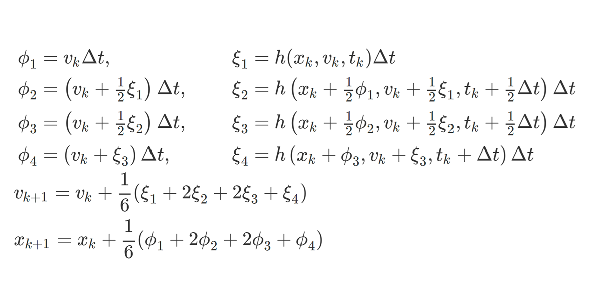
which is called the fourth-order Runge-Kutta method. These methods can be easily extended to second-order differential equations, and if we denote
\[ \small h(x_k,v_k,t_k) = f(x_k,t_k)v_k+g(x_k,t_k), \]
we can simply calculate it as follows:
\[ \small \begin{align*} &\begin{array}{ll} \phi_1 = v_k\Delta t, &\quad \xi_1 = h(x_k,v_k,t_k)\Delta t \\ \phi_2 = \left(v_k+\frac{1}{2}\xi_1\right)\Delta t, &\quad \xi_2 = h\left(x_k+\frac{1}{2}\phi_1,v_k+\frac{1}{2}\xi_1,t_k+\frac{1}{2}\Delta t\right)\Delta t \\ \phi_3 = \left(v_k+\frac{1}{2}\xi_2\right)\Delta t,& \quad \xi_3 = h\left(x_k+\frac{1}{2}\phi_2,v_k+\frac{1}{2}\xi_2,t_k+\frac{1}{2}\Delta t\right)\Delta t \\ \phi_4 = \left(v_k+\xi_3\right)\Delta t, &\quad \xi_4 = h\left(x_k+\phi_3,v_k+\xi_3,t_k+\Delta t\right)\Delta t \end{array}\\ &v_{k+1} = v_{k} + \frac{1}{6}(\xi_1+2\xi_2+2\xi_3+\xi_4) \\ &x_{k+1} = x_{k} + \frac{1}{6}(\phi_1+2\phi_2+2\phi_3+\phi_4). \end{align*} \]
In the case of the second-order Runge-Kutta method, it can be calculated as:
\[ \small \begin{align*} &v_{k+1} = v_{k} + \xi_2 \\ &x_{k+1} = x_{k} + \phi_2. \end{align*} \]
Differential equations are gradually becoming problems that cannot be solved, so I intend to use numerical methods to solve any problems that can be solved.

Comments